Parameter learning

Parameter learning is the task of estimating the values of Conditional Probability Distributions (CPDs). This process involves analyzing the frequency of variable states in the data. When variables are dependent on parent nodes, these counts are performed conditionally for each parent configuration.

Currently, the library supports parameter learning for discrete nodes using two main approaches:

1. Maximum Likelihood Estimation (MLE)

2. Bayesian Estimation

Maximum Likelihood Estimation

MLE estimates the parameters by maximizing the likelihood of the observed data. However, it can overfit the data, especially when dealing with small datasets.

While very straightforward, the ML estimator has the problem of overfitting to the data. If the observed data is not representative for the underlying distribution, ML estimations will be extremely far off. When estimating parameters for Bayesian networks, lack of data is a frequent problem. Even if the total sample size is very large, the fact that state counts are done conditionally for each parents configuration causes immense fragmentation. If a variable has 3 parents that can each take 10 states, then state counts will be done separately for 10^3 = 1000 parents configurations. This makes MLE very fragile and unstable for learning Bayesian Network parameters. A way to mitigate MLE’s overfitting is Bayesian Parameter Estimation.

Bayesian Parameter Estimation

Bayesian Parameter Estimation incorporates prior beliefs about the distributions of variables. This helps prevent overfitting and provides more robust parameter estimates.

One can think of the priors as consisting in pseudo state counts, that are added to the actual counts before normalization. Unless one wants to encode specific beliefs about the distributions of the variables, one commonly chooses uniform priors, i.e. ones that deem all states equiprobable.

A very simple prior is the so-called K2 prior, which simply adds “1” to the count of every single state. A somewhat more sensible choice of prior is BDeu (Bayesian Dirichlet equivalent uniform prior). For BDeu we need to specify an equivalent sample size “N” and then the pseudo-counts are the equivalent of having observed N uniform samples of each variable (and each parent configuration).

Parameter Learning Examples

Example 1: Sprinkler Dataset

For this example, we will be investigating the sprinkler dataset. This is a very simple dataset with 4 variables and each variable can contain value [1] or [0]. The question we can ask: What are the parameters for the DAG given a dataset? Note that this dataset is already pre-processed and no missing values are present. We need both a directed acyclic graph (DAG) and dataset with the same variables. The idea is to link the dataset with the DAG.

Let’s bring in our dataset:

import bnlearn
df = bnlearn.import_example()
df.head()

Cloudy	Sprinkler	Rain	Wet_Grass
0	1	0	1
1	1	1	1
1	0	1	1
…	…	…	…
0	0	0	0
1	0	0	0
1	0	1	1

Next, we import the DAG structure:

DAG = bnlearn.import_DAG('sprinkler', CPD=False)
print(DAG)

	Cloudy	Sprinkler	Rain	Wet_Grass
Cloudy	False	True	True	False
Sprinkler	False	False	False	True
Rain	False	False	False	True
Wet_Grass	False	False	False	False

Visualize the DAG:

bnlearn.plot(DAG)

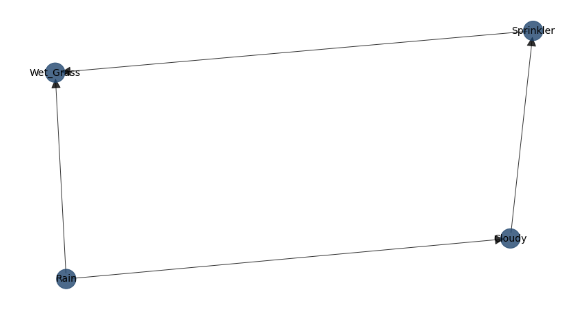
DAG of the Sprinkler dataset.

Suppose we observed N “cloudy” occurrences among a total of “all clouds”, so we might guess that about “50%” of “cloudy” are “sprinkler” or so. According to MLE, we should fill the CPDs in such a way, that P(data|model) is maximal. This is achieved when using the relative frequencies. From the bnlearn library, we’ll need the fit for this exercise:

DAG_update = bnlearn.parameter_learning.fit(DAG, df)

The learned CPDs are:

CPD of Cloudy:

Cloudy(0)	0.494
Cloudy(1)	0.506

CPD of Sprinkler:

Cloudy	Cloudy(0)	Cloudy(1)
Sprinkler(0)	0.48	0.70
Sprinkler(1)	0.51	0.29

CPD of Rain:

Cloudy	Cloudy(0)	Cloudy(1)
Rain(0)	0.65	0.33
Rain(1)	0.34	0.66

CPD of Wet_Grass:

Rain	Rain(0)	Rain(0)	Rain(1)	Rain(1)
Sprinkler	Sprinkler(0)	Sprinkler(1)	Sprinkler(0)	Sprinkler(1)
Wet_Grass(0)	0.75	0.33	0.25	0.37
Wet_Grass(1)	0.24	0.66	0.74	0.62

Great! We have the probabilities! Let’s check how much they differ from the truth. In general it can be seen that the estimated values are not very close at every point to the true values. The main reason is because the dataframe only contains 1000 samples.

DAG_true = bnlearn.import_DAG('sprinkler', CPD=True)

True CPDs:

CPD of Cloudy:

Cloudy(0)	0.5
Cloudy(1)	0.5

CPD of Sprinkler:

Cloudy	Cloudy(0)	Cloudy(1)
Sprinkler(0)	0.5	0.9
Sprinkler(1)	0.5	0.1

CPD of Rain:

Cloudy	Cloudy(0)	Cloudy(1)
Rain(0)	0.8	0.2
Rain(1)	0.2	0.8

CPD of Wet_Grass:

Sprinkler	Sprinkler(0)	Sprinkler(0)	Sprinkler(1)	Sprinkler(1)
Rain	Rain(0)	Rain(1)	Rain(0)	Rain(1)
Wet_Grass(0)	1.0	0.1	0.1	0.01
Wet_Grass(1)	0.0	0.9	0.9	0.99

Let’s generate more samples and learn again the parameters. You will see that these results are much closer to the true values.

df = bnlearn.sampling(DAG, n=10000)
DAG_update = bnlearn.parameter_learning.fit(DAG, df)

Example 2: Asia Dataset

Let’s try out a more complex model. We need both a directed acyclic graph (DAG) and dataset with the same variables. So again, the idea is to link the dataset with the DAG.

Let’s bring in the asia dataset:

import bnlearn

# Load asia dataset
DAG = bnlearn.import_DAG('asia')
# Plot
G = bnlearn.plot(DAG)

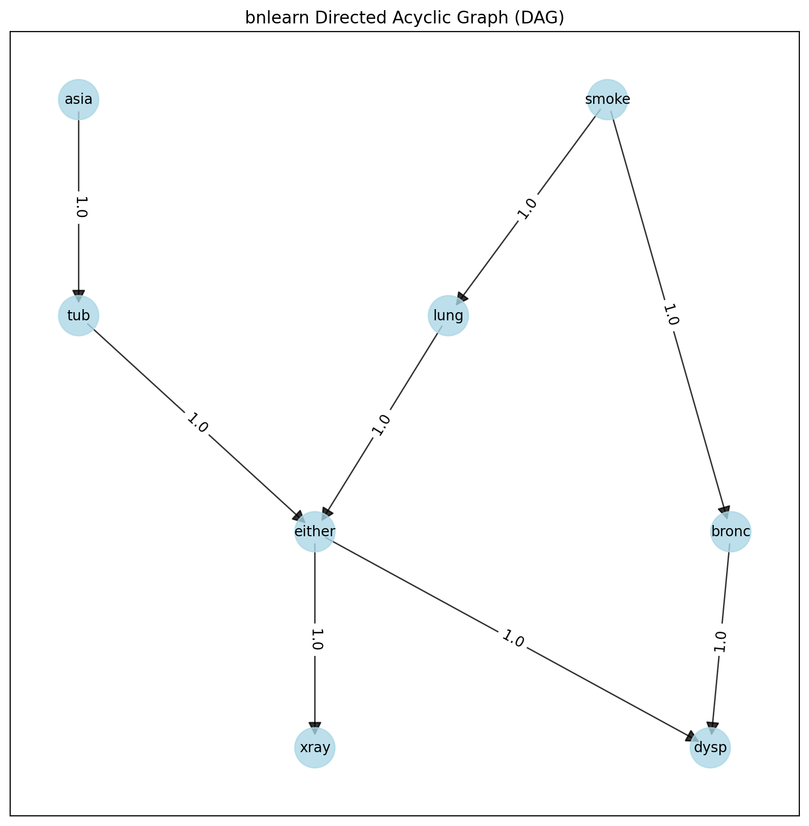
DAG of the Asia dataset.

# Generate samples
df = bnlearn.sampling(DAG, n=10000)

# Learn parameters
DAG_update = bnlearn.parameter_learning.fit(DAG, df)

This DAG is now updated with parameters which is great because it opens many possibilities in terms of inference or you can start sampling any number of samples you desire.

CPD of asia:

asia(0)	0.055
asia(1)	0.944

CPD of bronc:

smoke	smoke(0)	smoke(1)
bronc(0)	0.585	0.319
bronc(1)	0.414	0.680

CPD of dysp:

bronc	bronc(0)	bronc(0)	bronc(1)	bronc(1)
either	either(0)	either(1)	either(0)	either(1)
dysp(0)	0.714	0.787	0.586	0.123
dysp(1)	0.285	0.212	0.413	0.876

CPD of either:

lung	lung(0)	lung(0)	lung(1)	lung(1)
tub	tub(0)	tub(1)	tub(0)	tub(1)
either(0)	0.507	0.837	0.642	0.012
either(1)	0.492	0.1625	0.357	0.987

CPD of lung:

smoke	smoke(0)	smoke(1)
lung(0)	0.132	0.0537
lung(1)	0.867	0.9462

CPD of smoke:

smoke(0)	0.498
smoke(1)	0.501

CPD of tub:

asia	asia(0)	asia(1)
tub(0)	0.418	0.0336
tub(1)	0.581	0.9663

CPD of xray:

either	either(0)	either(1)
xray(0)	0.7693	0.070
xray(1)	0.230	0.929

Conditional Probability Distributions (CPD)

The Conditional Probabilistic Tables (CPTs) or Conditional Probability Distributions (CPD) quantitatively describe the statistical relationship between each node and its parents, and can be computed using Parameter learning as shown in the examples. In the following example I will show how to extract the CPDs from a model.

# Import library
import bnlearn as bn

# Import one of the example models
# sprinkler', 'alarm', 'andes', 'asia', 'sachs', 'filepath/to/model.bif',
model = bn.import_DAG('asia', CPD=True)

# Print the CPD for the model
CPDs = bn.print_CPD(model)

# Deeper investigate the CPDs
CPDs.keys()
# dict_keys(['asia', 'bronc', 'dysp', 'either', 'lung', 'smoke', 'tub', 'xray'])

print(CPDs['smoke'])
#    smoke    p
# 0      0  0.5
# 1      1  0.5

---

---