Directed Acyclic Graphs
This section describes how to design your Directed Acyclic Graphs (DAGs), and how to assign Conditional Probability Distributions (CPDs).
Build a DAG (Auto generated CPTs)
Build a DAG (Manual CPTs)
Inference on the causal generative model
Build a DAG (Auto generated CPTs)
If you already know the relationships between variables—either through prior knowledge or domain expertise—you can define the (causal) dependencies directly using a Directed Acyclic Graph (DAG).
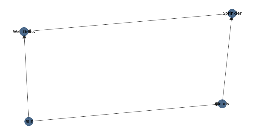
In a DAG: - Each node represents a variable. - Each directed edge represents a direct dependency (often causal) from one variable to another.
In bnlearn, we can explicitly construct and visualize these relationships. Below, we demonstrate this with the classic Sprinkler example. First, we define the directed relationships between the variables by specifying the edges:
Cloudy -> Sprinkler
Cloudy -> Rain
Sprinkler -> Wet_Grass
Rain -> Wet_Grass
# Import the library
import bnlearn as bn

# Define the network structure
edges = [('Cloudy', 'Sprinkler'),
         ('Cloudy', 'Rain'),
         ('Sprinkler', 'Wet_Grass'),
         ('Rain', 'Wet_Grass')]

# Make the Bayesian DAG. The CPTs are auto-generated.
DAG = bn.make_DAG(edges, methodtype='bayes')

# Plot the DAG
bn.plot(DAG)

# Print the CPD
d = bn.print_CPD(DAG)
We call this a causal DAG because we have assumed that the edges we encoded represent our causal assumptions about the system. When using bnlearn.make_DAG, the Conditional Probability Tables (CPTs), also known as Conditional Probability Distributions (CPDs), are automatically generated for all nodes if not explicitly provided.
- These default CPTs assume:
A uniform probability distribution, meaning that all outcomes are equally likely.
A default cardinality (variable_card) of 2, meaning that each node two has two states, [0, 1].
You can override these defaults by explicitly specifying custom CPTs using TabularCPD from pgmpy.
Alternatively, you can generate them using bnlearn.generate_cpt() for greater control over cardinality and probability values.
# Import the library
import bnlearn as bn

# Define the network structure
edges = [('Cloudy', 'Sprinkler'),
         ('Cloudy', 'Rain'),
         ('Sprinkler', 'Wet_Grass'),
         ('Rain', 'Wet_Grass')]

# Generate Placeholder CPTs
CPD = bn.build_cpts_from_structure(edges, variable_card=3)

# Adjust the Probability Table(s) accordingly
CPD[0].values

# Create the DAG and add the probabiilty tables (CPD)
model = bn.make_DAG(edges, CPD=CPD)

# Print the CPD
d = bn.print_CPD(model)

# Make inferences
q = bn.inference.fit(model, variables=['Wet_Grass'], evidence={'Rain': 1, 'Sprinkler': 0, 'Cloudy': 1})


[bnlearn] >Variable Elimination.
+----+-------------+----------+
|    |   Wet_Grass |        p |
+====+=============+==========+
|  0 |           0 | 0.333333 |
+----+-------------+----------+
|  1 |           1 | 0.333333 |
+----+-------------+----------+
|  2 |           2 | 0.333333 |
+----+-------------+----------+

Summary for variables: ['Wet_Grass']
Given evidence: Rain=1, Sprinkler=0, Cloudy=1

Wet_Grass outcomes:
- Wet_Grass: 0 (33.3%)
- Wet_Grass: 1 (33.3%)
- Wet_Grass: 2 (33.3%)
We can have more controle per node and the variable_card and probabilities as following. Note that if you change the variable_card, it must also match with the child nodes, otherwise it will return a cardinality error!
# Import the library
import bnlearn as bn

# Define the network structure
edges = [('Cloudy', 'Sprinkler'),
         ('Cloudy', 'Rain'),
         ('Sprinkler', 'Wet_Grass'),
         ('Rain', 'Wet_Grass')]

# Get parent nodes from the edges
parents = bn.get_parents(edges)

print(parents)
{'Sprinkler': ['Cloudy'],
 'Rain': ['Cloudy'],
 'Wet_Grass': ['Sprinkler', 'Rain'],
 'Cloudy': []}

# Create the CPT for each node. When changing the variable_card, it should match the cardinality!
cpt_cloudy = bn.generate_cpt('Cloudy', parents.get('Cloudy'), variable_card=2)
cpt_sprinkler = bn.generate_cpt('Sprinkler', parents.get('Sprinkler'), variable_card=2)
cpt_rain = bn.generate_cpt('Rain', parents.get('Rain'), variable_card=2)
cpt_wetgrass = bn.generate_cpt('Wet_Grass', parents.get('Wet_Grass'), variable_card=2)

# Create the DAG with custom CPTs. The order of the CPTs does not matter.
model = bn.make_DAG(edges, CPD=[cpt_sprinkler, cpt_rain, cpt_wetgrass, cpt_cloudy])

# The causal DAG as a generative representation of joint probability
d = bn.print_CPD(model)

# Make inferences
q = bn.inference.fit(model, variables=['Wet_Grass'], evidence={'Rain': 1, 'Sprinkler': 0, 'Cloudy': 1})
Build a DAG (Manual CPTs)
Each factor in a Bayesian network is a conditional probability distribution (CPD), often referred to as a conditional probability table (CPT) in the discrete case. While CPDs can be derived from any directed acyclic graph (DAG), if the DAG represents causal relationships, the resulting CPDs are better interpreted as causal Markov kernels (CMKs). This causal factorization is particularly valuable because each CMK reflects an independent causal mechanism—assumed to remain stable across different datasets. Despite this distinction, the term CPD is still more commonly used than CMK.
For each node we can specify the probability distributions as following:
# Import the library
import bnlearn as bn

# Define the network structure
edges = [('Cloudy', 'Sprinkler'),
         ('Cloudy', 'Rain'),
         ('Sprinkler', 'Wet_Grass'),
         ('Rain', 'Wet_Grass')]

# Import the library
from pgmpy.factors.discrete import TabularCPD

# Cloudy has no parents
cpt_cloudy = TabularCPD(variable='Cloudy', variable_card=3,
                        values=[[0.2], [0.3], [0.5]])

# Sprinkler | Cloudy (Cloudy has 3 values)
cpt_sprinkler = TabularCPD(variable='Sprinkler', variable_card=2,
                           values=[[0.9, 0.6, 0.1],  # Sprinkler=0
                                   [0.1, 0.4, 0.9]], # Sprinkler=1
                           evidence=['Cloudy'], evidence_card=[3])

# Rain | Cloudy (Cloudy has 3 values)
cpt_rain = TabularCPD(variable='Rain', variable_card=2,
                      values=[[0.8, 0.5, 0.2],  # Rain=0
                              [0.2, 0.5, 0.8]], # Rain=1
                      evidence=['Cloudy'], evidence_card=[3])

# Wet_Grass | Sprinkler, Rain (both binary)
cpt_wetgrass = TabularCPD(variable='Wet_Grass', variable_card=2,
                          values=[[1.0, 0.1, 0.1, 0.01],  # Wet_Grass=0
                                  [0.0, 0.9, 0.9, 0.99]], # Wet_Grass=1
                          evidence=['Sprinkler', 'Rain'], evidence_card=[2, 2])

print(cpt_sprinkler)
print(cpt_rain)
print(cpt_wet_grass)
print(cpt_cloudy)
# +-----------+-----+
# | Cloudy(0) | 0.3 |
# +-----------+-----+
# | Cloudy(1) | 0.7 |
# +-----------+-----+

# Now need to connect the edges with CPDs.
model = bn.make_DAG(edges, CPD=[cpt_cloudy, cpt_sprinkler, cpt_rain, cpt_wet_grass])

# The causal DAG as a generative representation of joint probability
d = bn.print_CPD(model)

# Make inferences
q = bn.inference.fit(model, variables=['Wet_Grass'], evidence={'Rain': 1, 'Sprinkler': 0, 'Cloudy': 1})