Modelling Continuous Datasets

Learning Bayesian Networks from continuous data is a challenging task. There are different approaches to working with continuous and/or hybrid datasets, each with its own advantages and disadvantages.

In bnlearn, the following options are available to work with continuous datasets:

1. Discretize continuous datasets manually using domain knowledge

2. Discretize continuous datasets using probability density fitting

3. Discretize continuous datasets using a principled Bayesian discretization method

4. Model continuous and hybrid datasets in a semi-parametric approach that assumes linear relationships

LiNGAM-based Methods

Bnlearn includes LiNGAM-based methods which estimate Linear, Non-Gaussian Acyclic Models from observed data. These methods assume non-Gaussianity of the noise terms in the causal model. Various methods have been developed and published, of which Bnlearn includes two: ICA-based LiNGAM [1] and DirectLiNGAM [2]. The following three methods are not included: VAR-LiNGAM [3], RCD [4], and CAM-UV [5].

[1]

Shimizu, S., Hoyer, P. O., Hyvarinen, A., Kerminen, A., & Jordan, M. (2006). A linear non-Gaussian acyclic model for causal discovery. Journal of Machine Learning Research, 7(10).

[2]

Shimizu, S., Inazumi, T., Sogawa, Y., Hyvarinen, A., Kawahara, Y., Washio, T., … & Bollen, K. (2011). DirectLiNGAM: A direct method for learning a linear non-Gaussian structural equation model. The Journal of Machine Learning Research, 12, 1225-1248.

[3]

Hyvarinen, A., Zhang, K., Shimizu, S., & Hoyer, P. O. (2010). Estimation of a structural vector autoregression model using non-gaussianity. Journal of Machine Learning Research, 11(5).

[4]

Maeda, T. N., & Shimizu, S. (2020, June). RCD: Repetitive causal discovery of linear non-Gaussian acyclic models with latent confounders. In International Conference on Artificial Intelligence and Statistics (pp. 735-745). PMLR.

[5]

Maeda, T. N., & Shimizu, S. (2021). Causal Additive Models with Unobserved Variables. UAI.

Toy Example

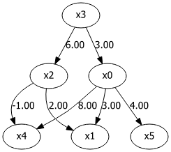
To demonstrate how LiNGAM works, let’s create a small toy example with six variables. The goal of this dataset is to demonstrate the contribution of different variables and their causal impact on other variables. All variables must be consistent, as in any other dataset. The sample size is set to n=1000 with a uniform distribution. If the number of samples is much smaller (e.g., in the tens), the method becomes less reliable due to insufficient information to determine causality.

We will establish dependencies between variables and then allow the model to infer the original values:

1. Step 1: x3 is the root node and is initialized with a uniform distribution.

2. Step 2: x0 and x2 are created by multiplying with the values of x3, making them dependent on x3.

3. Step 3: x5 is created by multiplying with the values of x0, making it dependent on x0.

4. Step 4: x1 and x4 are created by multiplying with the values of x0, making them dependent on x0.

import numpy as np
import pandas as pd
from lingam.utils import make_dot

# Number of samples
n = 1000

# Step 1: Initialize root node
x3 = np.random.uniform(size=n)

# Step 2: Create dependent variables
x0 = 3.0 * x3 + np.random.uniform(size=n)
x2 = 6.0 * x3 + np.random.uniform(size=n)

# Step 3: Create further dependencies
x5 = 4.0 * x0 + np.random.uniform(size=n)

# Step 4: Create final dependencies
x1 = 3.0 * x0 + 2.0 * x2 + np.random.uniform(size=n)
x4 = 8.0 * x0 - 1.0 * x2 + np.random.uniform(size=n)

# Create DataFrame
df = pd.DataFrame(np.array([x0, x1, x2, x3, x4, x5]).T,
                 columns=['x0', 'x1', 'x2', 'x3', 'x4', 'x5'])
df.head()

# Define adjacency matrix
m = np.array([[0.0, 0.0, 0.0, 3.0, 0.0, 0.0],
             [3.0, 0.0, 2.0, 0.0, 0.0, 0.0],
             [0.0, 0.0, 0.0, 6.0, 0.0, 0.0],
             [0.0, 0.0, 0.0, 0.0, 0.0, 0.0],
             [8.0, 0.0,-1.0, 0.0, 0.0, 0.0],
             [4.0, 0.0, 0.0, 0.0, 0.0, 0.0]])
dot = make_dot(m)
dot

Structure learning can be applied with the direct-lingam method for fitting:

# Fit the model
model = bn.structure_learning.fit(df, methodtype='direct-lingam')

# Examine the output to see how well the dependency values are recovered
print(model['adjmat'])
# target        x0        x1       x2   x3        x4       x5
# source
# x0      0.000000  2.987320  0.00000  0.0  8.057757  3.99624
# x1      0.000000  0.000000  0.00000  0.0  0.000000  0.00000
# x2      0.000000  2.010043  0.00000  0.0 -0.915306  0.00000
# x3      2.971198  0.000000  5.98564  0.0 -0.704964  0.00000
# x4      0.000000  0.000000  0.00000  0.0  0.000000  0.00000
# x5      0.000000  0.000000  0.00000  0.0  0.000000  0.00000

# Visualize the model
bn.plot(model)

# Compute edge strength with chi-square test statistic
model = bn.independence_test(model, df, prune=False)

print(model['adjmat'])
# target        x0        x1       x2   x3        x4       x5
# source
# x0      0.000000  2.987320  0.00000  0.0  8.057757  3.99624
# x1      0.000000  0.000000  0.00000  0.0  0.000000  0.00000
# x2      0.000000  2.010043  0.00000  0.0 -0.915306  0.00000
# x3      2.971198  0.000000  5.98564  0.0 -0.704964  0.00000
# x4      0.000000  0.000000  0.00000  0.0  0.000000  0.00000
# x5      0.000000  0.000000  0.00000  0.0  0.000000  0.00000

# Examine the causal ordering
print(model['causal_order'])
# ['x3', 'x0', 'x5', 'x2', 'x1', 'x4']

# Visualize the causal graph
bn.plot(model)

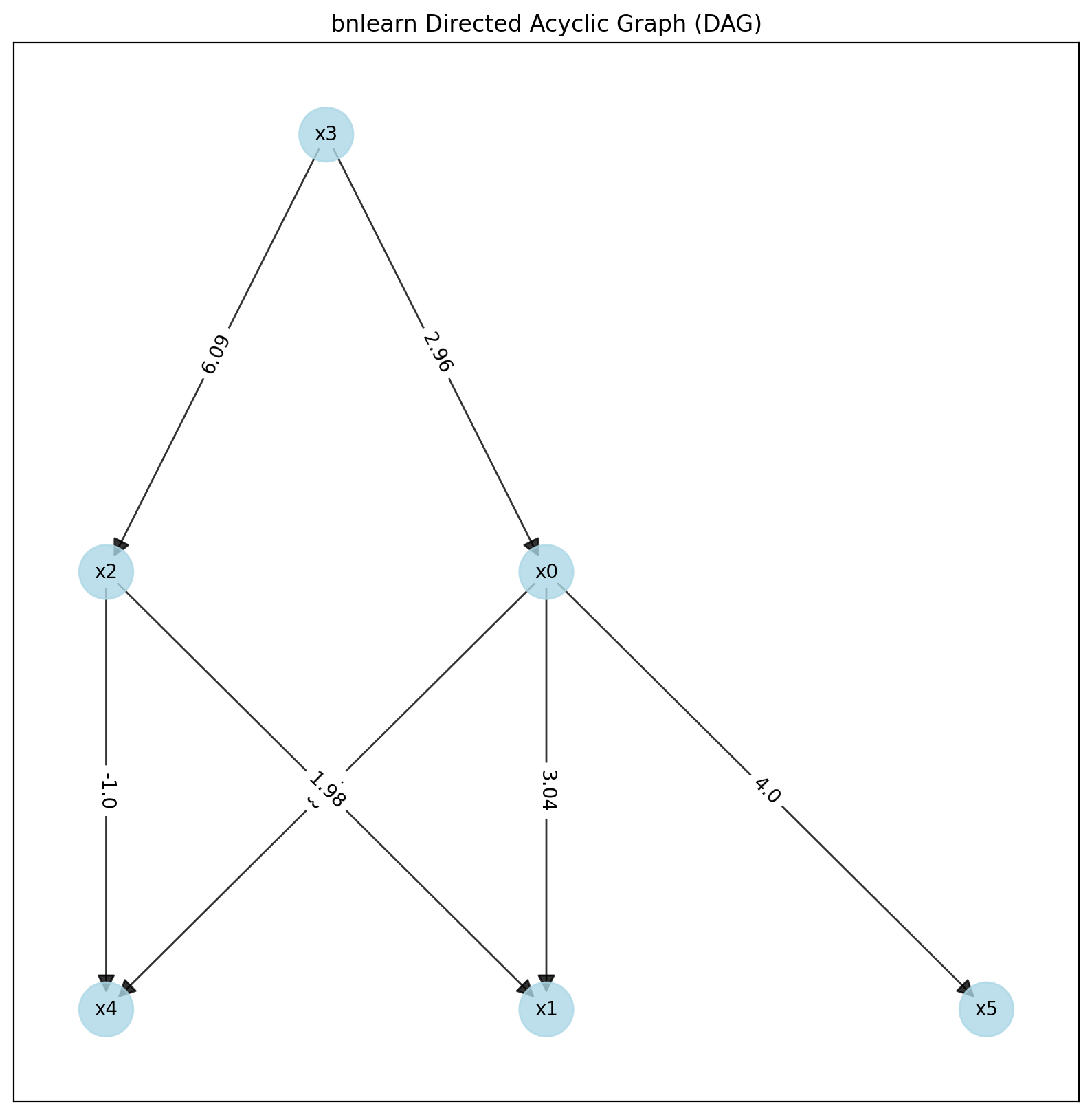
This example nicely demonstrates that we can accurately capture the dependencies with the causal factors.

Direct-LiNGAM Method

The Direct-LiNGAM method ‘direct-lingam’ is a semi-parametric approach that assumes a linear relationship among observed variables while ensuring that the error terms follow a non-Gaussian distribution, with the constraint that the graph remains acyclic. This method involves repeated regression analysis and independence assessments using linear regression with least squares. In each regression, one variable serves as the dependent variable (outcome), while the other acts as the independent variable (predictor). This process is applied to each type of variable. When regression analysis is conducted in the correct causal order, the independent variables and error terms will exhibit independence. Conversely, if the regression is performed under an incorrect causal order, the independence of the explanatory variables and error terms is disrupted. By leveraging the dependency properties (where both residuals and explanatory variables share common error terms), it becomes possible to infer the causal order among the variables. Furthermore, for a given observed variable, any explanatory variable that remains independent of the residuals, regardless of the other variables considered, can be inferred as the first in the causal hierarchy.

When regression analysis is conducted in the correct causal order, the independent variables and error terms will exhibit independence. Conversely, if the regression is performed under an incorrect causal order, the independence of the explanatory variables and error terms is disrupted. By leveraging the dependency properties (where both residuals and explanatory variables share common error terms), it becomes possible to infer the causal order among the variables. Furthermore, for a given observed variable, any explanatory variable that remains independent of the residuals, regardless of the other variables considered, can be inferred as the first in the causal hierarchy.

In other words, the lingam-direct method allows you to model continuous and mixed datasets. A limitation is that causal discovery of structure learning is the endpoint when using this method. It is not possible to perform parameter learning and inferences.

# Import libraries
import bnlearn as bn

# Load dataset
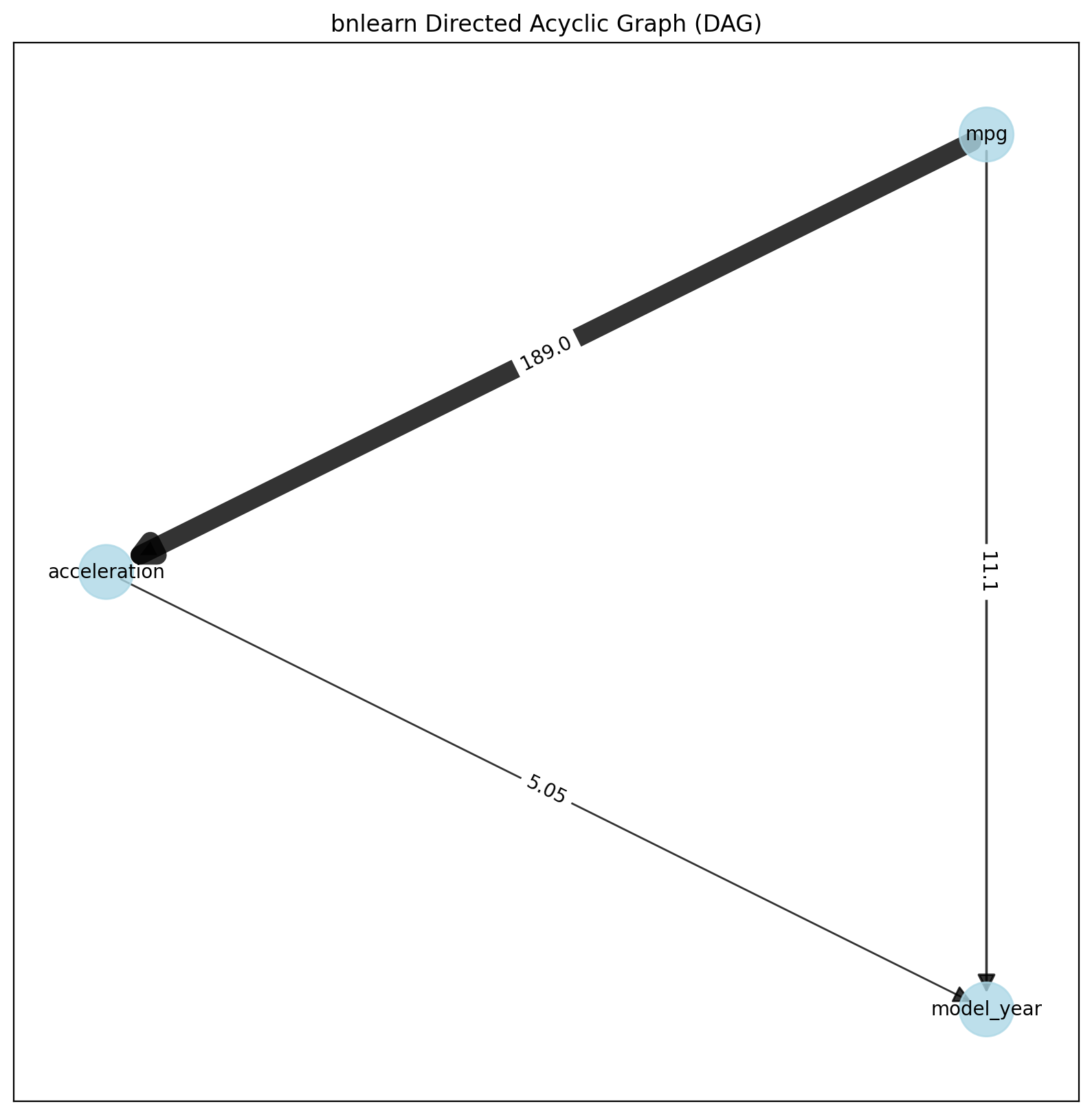
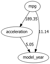
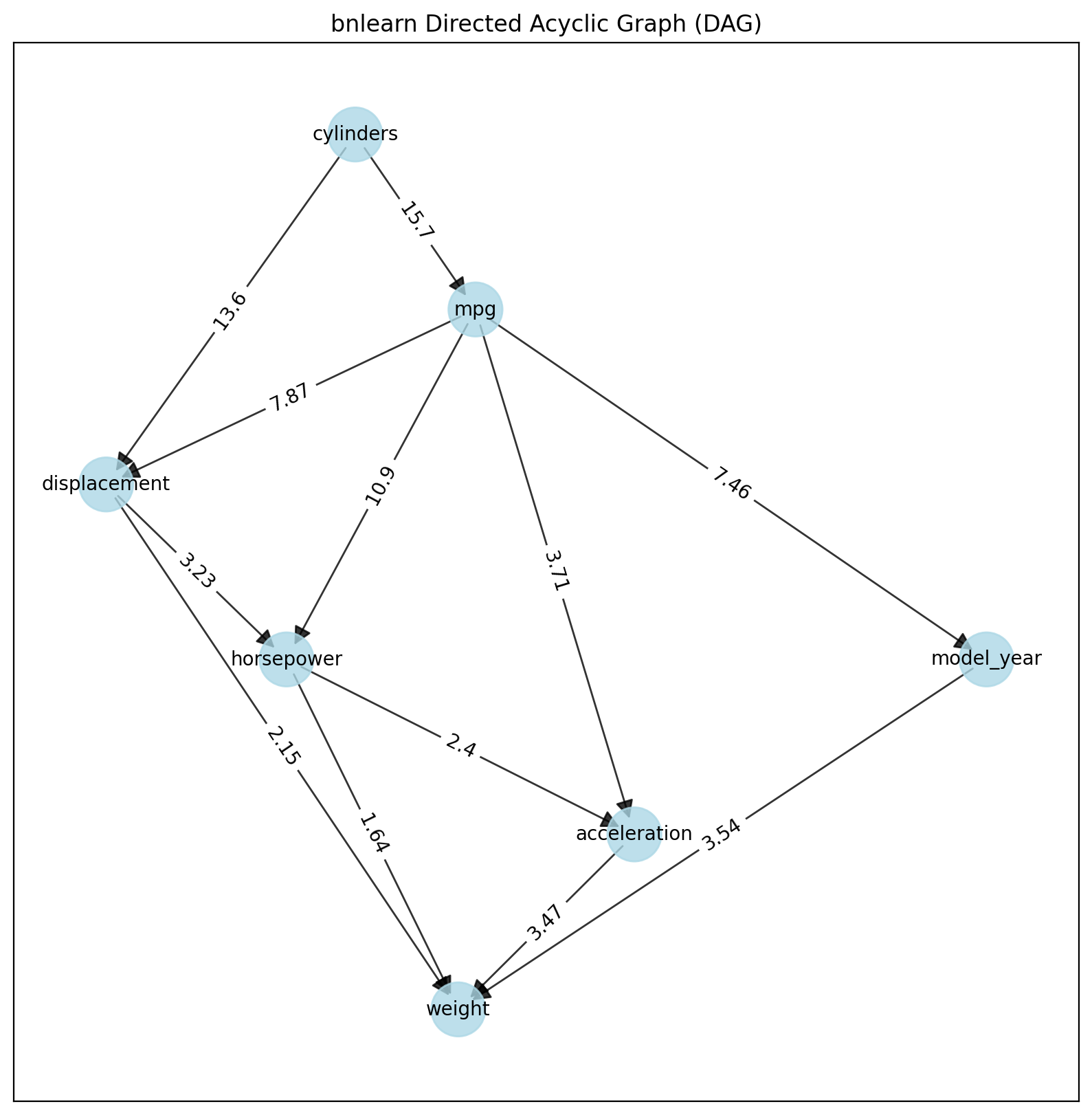
df = bn.import_example(data='auto_mpg')
del df['origin']

# Perform structure learning
model = bn.structure_learning.fit(df,
                                methodtype='direct-lingam',
                                params_lingam={'random_state': 2})

# Compute edge strength
model = bn.independence_test(model, df, prune=True)

# Create visualizations
bn.plot(model)
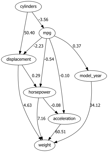
dotgraph = bn.plot_graphviz(model)
dotgraph
dotgraph.view(filename=r'dotgraph_auto_mpg_lingam_direct')

Using the LINGAM method, the values on the edges describe the dependency using a multiplication factor of one variable to another. For example, Origin -> -10 -> Displacement tells us that Displacement has values that are a factor of -10 lower than origin.

ICA-LiNGAM Method

The ICA-LiNGAM method (‘ica-lingam’) is also from lingam and follows the same procedure.

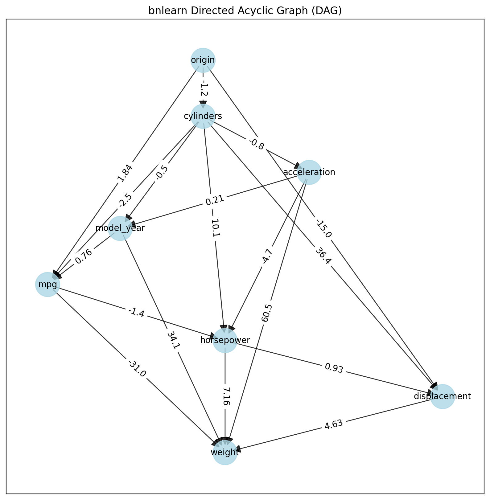
# Import libraries
import bnlearn as bn

# Load dataset
df = bn.import_example(data='auto_mpg')
del df['origin']

# Perform structure learning
model = bn.structure_learning.fit(df, methodtype='ica-lingam')

# Compute edge strength
model = bn.independence_test(model, df, prune=True)

# Create visualizations
bn.plot(model)
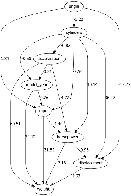
dotgraph = bn.plot_graphviz(model)
dotgraph
dotgraph.view(filename=r'dotgraph_auto_mpg_lingam_ica')

PC Method

A different, but quite straightforward approach to building a DAG from data is identifying independencies in the dataset using hypothesis tests and then constructing a DAG (pattern) according to the identified independencies (Conditional Independence Tests). Independencies in the data can be identified using chi2 conditional independence tests.

The Constraint-Based PC Algorithm (named after Peter and Clark, its inventors) is a popular method in causal inference and Bayesian network learning. It is a type of constraint-based algorithm that uses conditional independence tests to build a causal graph from data. This algorithm is widely used to learn the structure of Bayesian networks and causal graphs by identifying relationships between variables.

DAG (pattern) construction involves three steps: 1. Construct an undirected skeleton 2. Orient compelled edges to obtain a partially directed acyclic graph 3. Extend the DAG pattern to a DAG by conservatively orienting the remaining edges

# Import libraries
import bnlearn as bn

# Load dataset
df = bn.import_example(data='auto_mpg')

# Perform structure learning
model = bn.structure_learning.fit(df, methodtype='pc')

# Compute edge strength
model = bn.independence_test(model, df, prune=True)

# Create visualizations
bn.plot(model)
dotgraph = bn.plot_graphviz(model)
dotgraph
dotgraph.view(filename=r'dotgraph_auto_mpg_PC')

PC PDAG construction is only guaranteed to work under the assumption that the identified set of independencies is faithful, i.e. there exists a DAG that exactly corresponds to it. Spurious dependencies in the data set can cause the reported independencies to violate faithfulness. It can happen that the estimated PDAG does not have any faithful completions (i.e. edge orientations that do not introduce new v-structures). In that case a warning is issued.

---

---