Examples

bnlearn contains several examples within the library that can be used to practice with the functionalities of bnlearn.structure_learning(), bnlearn.parameter_learning(), and bnlearn.inference().

Working with Raw Data

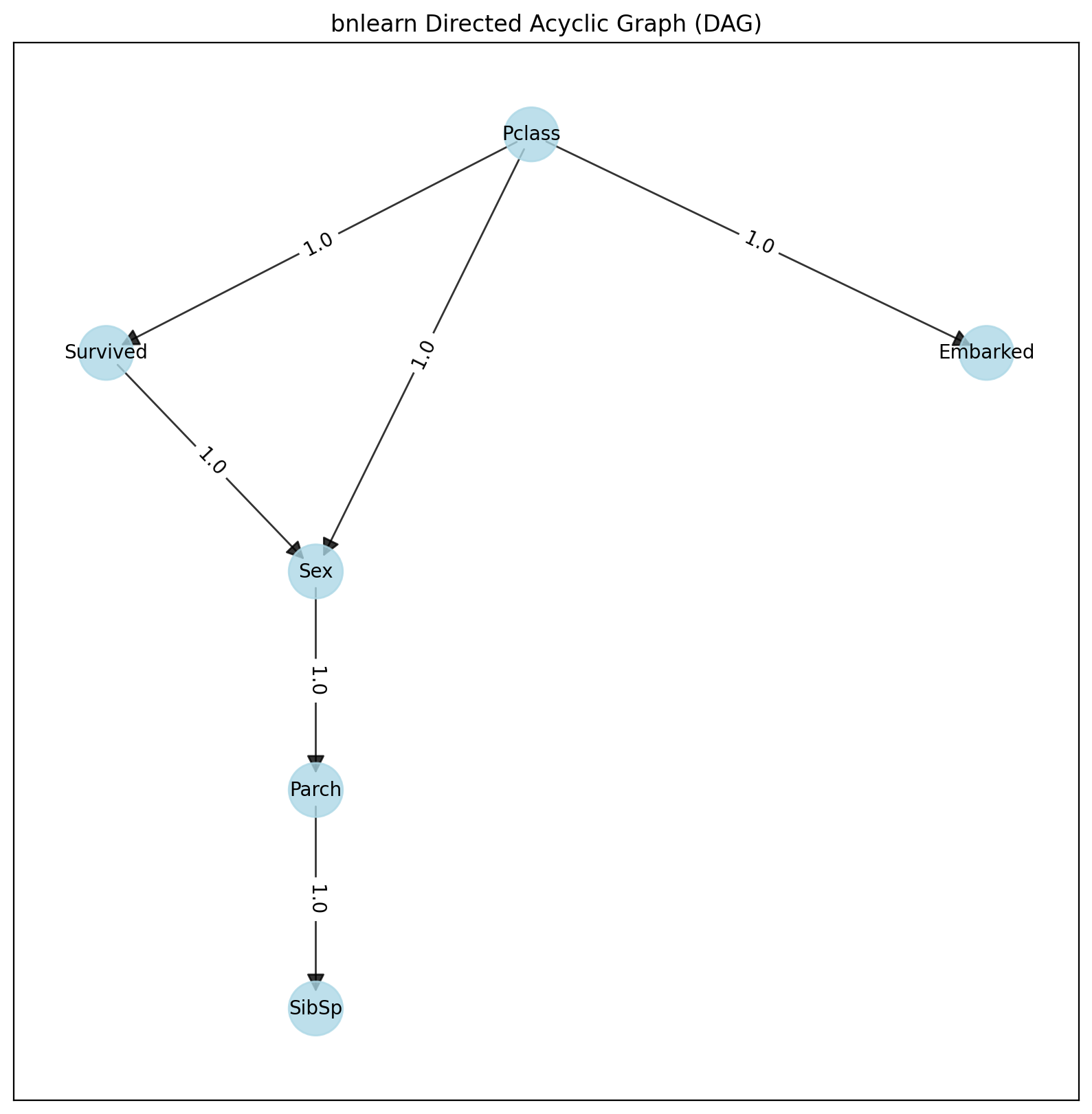
Let’s demonstrate how to process a dataset containing mixed variables using the Titanic dataset as an example. This dataset contains both continuous and categorical variables and can be easily imported using bnlearn.bnlearn.import_example(). The function bnlearn.bnlearn.df2onehot() helps convert the mixed dataset into a one-hot matrix. By default, the unique non-zero values must be above 80% per variable, and the minimum number of samples must be at least 10 per variable.

import bnlearn as bn
# Load Titanic dataset containing mixed variables
df_raw = bn.import_example(data='titanic')

# Pre-process the input dataset
dfhot, dfnum = bn.df2onehot(df_raw)

# Structure learning
DAG = bn.structure_learning.fit(dfnum)

# Plot
G = bn.plot(DAG)
bn.plot_graphviz(DAG)

From this point, we can learn the parameters using the DAG and input dataframe:

# Parameter learning
model = bn.parameter_learning.fit(DAG, dfnum)

Finally, we can start making inferences. Note that the variable and evidence names should exactly match the input data (case sensitive):

# Print CPDs
CPDs = bn.print_CPD(model)
# Make inference
q = bn.inference.fit(model, variables=['Survived'], evidence={'Sex':0, 'Pclass':1})

print(q.df)
print(q._str())

Survived	phi(Survived)
Survived(0)	0.3312
Survived(1)	0.6688

Structure Learning Example

A different but straightforward approach to build a DAG from data is to identify independencies in the dataset using hypothesis tests, such as the chi-square test statistic. The p-value of the test and a heuristic flag indicate if the sample size was sufficient. The p-value is the probability of observing the computed chi-square statistic (or an even higher chi-square value), given the null hypothesis that X and Y are independent given Zs. This can be used to make independence judgments at a given significance level.

Example 1: Basic Structure Learning

import bnlearn as bn
# Load dataframe
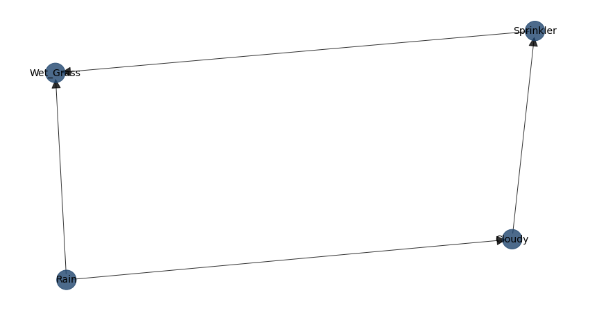
df = bn.import_example()
# Learn structure
model = bn.structure_learning.fit(df)
# Get adjacency matrix
model['adjmat']

# Print adjacency matrix
print(model['adjmat'])

Reading the table from left to right: - Cloudy is connected to Sprinkler and Rain in a directed manner - Sprinkler is connected to Wet_grass - Rain is connected to Wet_grass - Wet_grass has no outgoing connections

	Cloudy	Sprinkler	Rain	Wet_Grass
Cloudy	False	True	True	False
Sprinkler	False	False	False	True
Rain	False	False	False	True
Wet_Grass	False	False	False	False

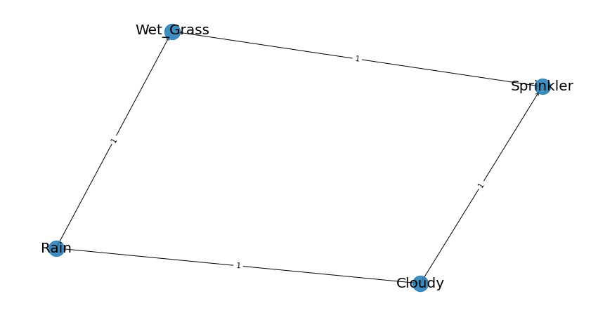
Example 2: Sprinkler Dataset

For this example, we will investigate the sprinkler dataset. This is a simple dataset with 4 variables, where each variable can contain values [1] or [0]. The question we can ask is: What are the relationships and dependencies across the variables? Note that this dataset is already pre-processed and contains no missing values.

Let’s load our dataset:

import bnlearn as bn
df = bn.import_example()
df.head()

Cloudy	Sprinkler	Rain	Wet_Grass
0	1	0	1
1	1	1	1
1	0	1	1
…	…	…	…
0	0	0	0
1	0	0	0
1	0	1	1

From the bnlearn library, we’ll use the fit function:

import bnlearn as bn
model = bn.structure_learning.fit(df)
G = bn.plot(model)
dot = bn.plot_graphviz(DAG)

Learned structure on the Sprinkler dataset

We can specify the method and scoring type. As described previously, some methods are more computationally expensive than others. Choose based on: - Number of variables - Available hardware - Time constraints

Method types: * hillclimbsearch or hc (greedy local search for networks with many nodes) * exhaustivesearch or ex (exhaustive search for very small networks) * constraintsearch or cs (Constraint-based Structure Learning using hypothesis tests)

Scoring types: * bic (Bayesian Information Criterion) * k2 (K2 score) * bdeu (Bayesian Dirichlet equivalent uniform)

import bnlearn as bn
model_hc_bic  = bn.structure_learning.fit(df, methodtype='hc', scoretype='bic')
model_hc_k2   = bn.structure_learning.fit(df, methodtype='hc', scoretype='k2')
model_hc_bdeu = bn.structure_learning.fit(df, methodtype='hc', scoretype='bdeu')
model_ex_bic  = bn.structure_learning.fit(df, methodtype='ex', scoretype='bic')
model_ex_k2   = bn.structure_learning.fit(df, methodtype='ex', scoretype='k2')
model_ex_bdeu = bn.structure_learning.fit(df, methodtype='ex', scoretype='bdeu')

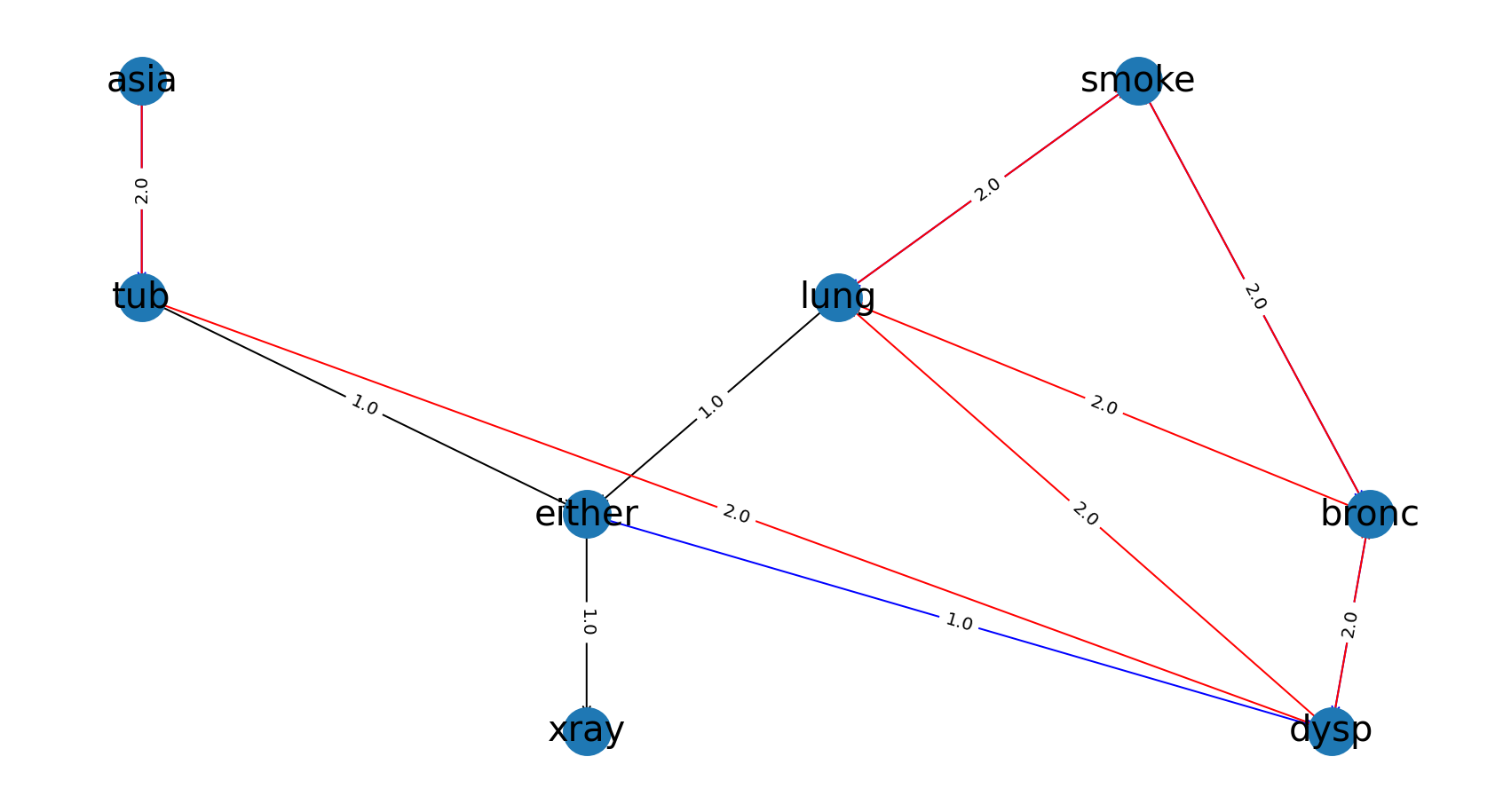
Example 3: Asia Dataset

Let’s learn the structure of a more complex dataset and compare it to another one:

import bnlearn as bn
# Load Asia DAG
model_true = bn.import_DAG('asia')
# Plot ground truth
G = bn.plot(model_true)
dot = bn.plot_graphviz(model_true)

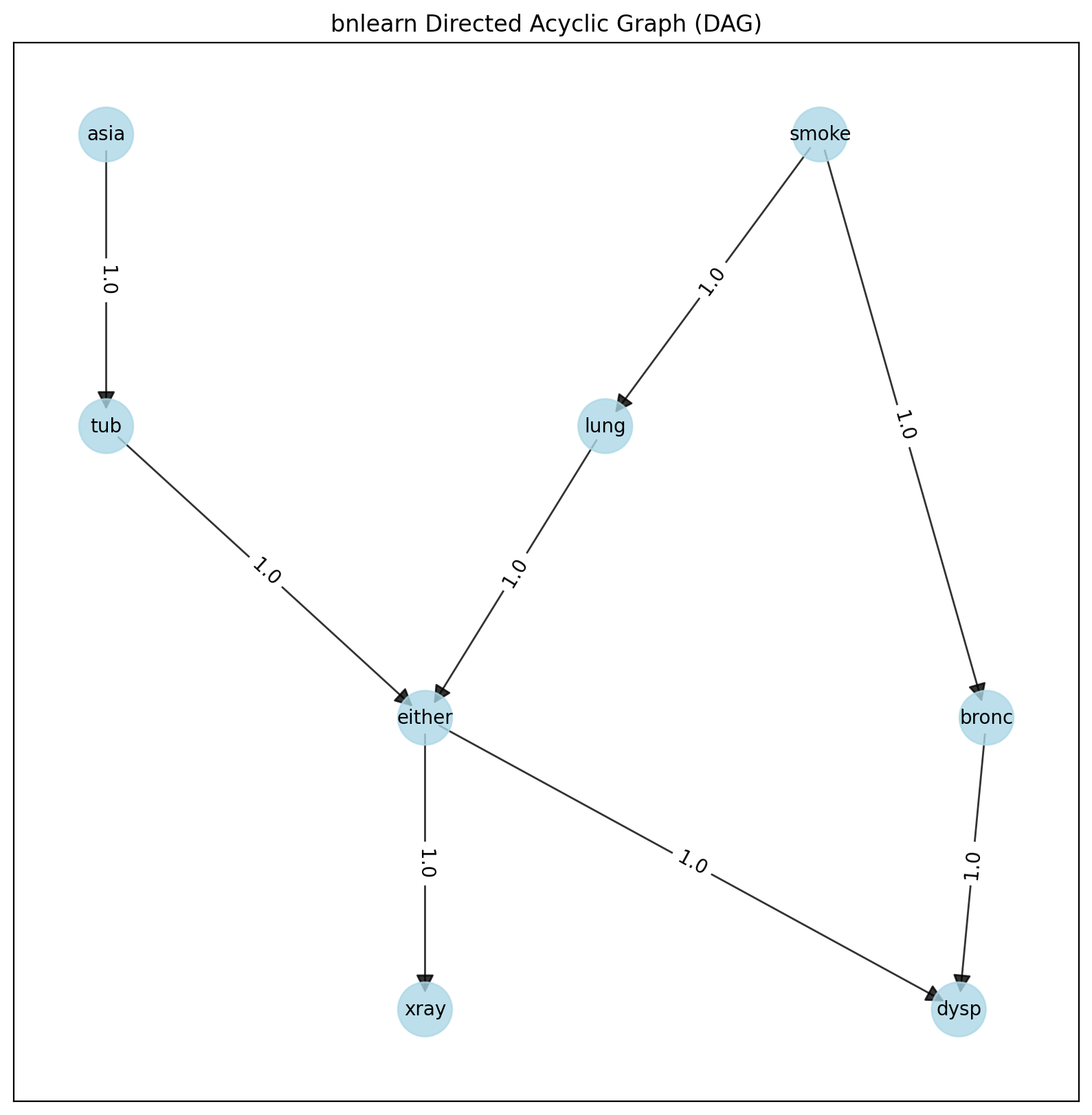
True DAG of the Asia dataset.

# Generate samples
df = bn.sampling(model_true, n=10000)
# Structure learning of sampled dataset
model_learned = bn.structure_learning.fit(df, methodtype='hc', scoretype='bic')

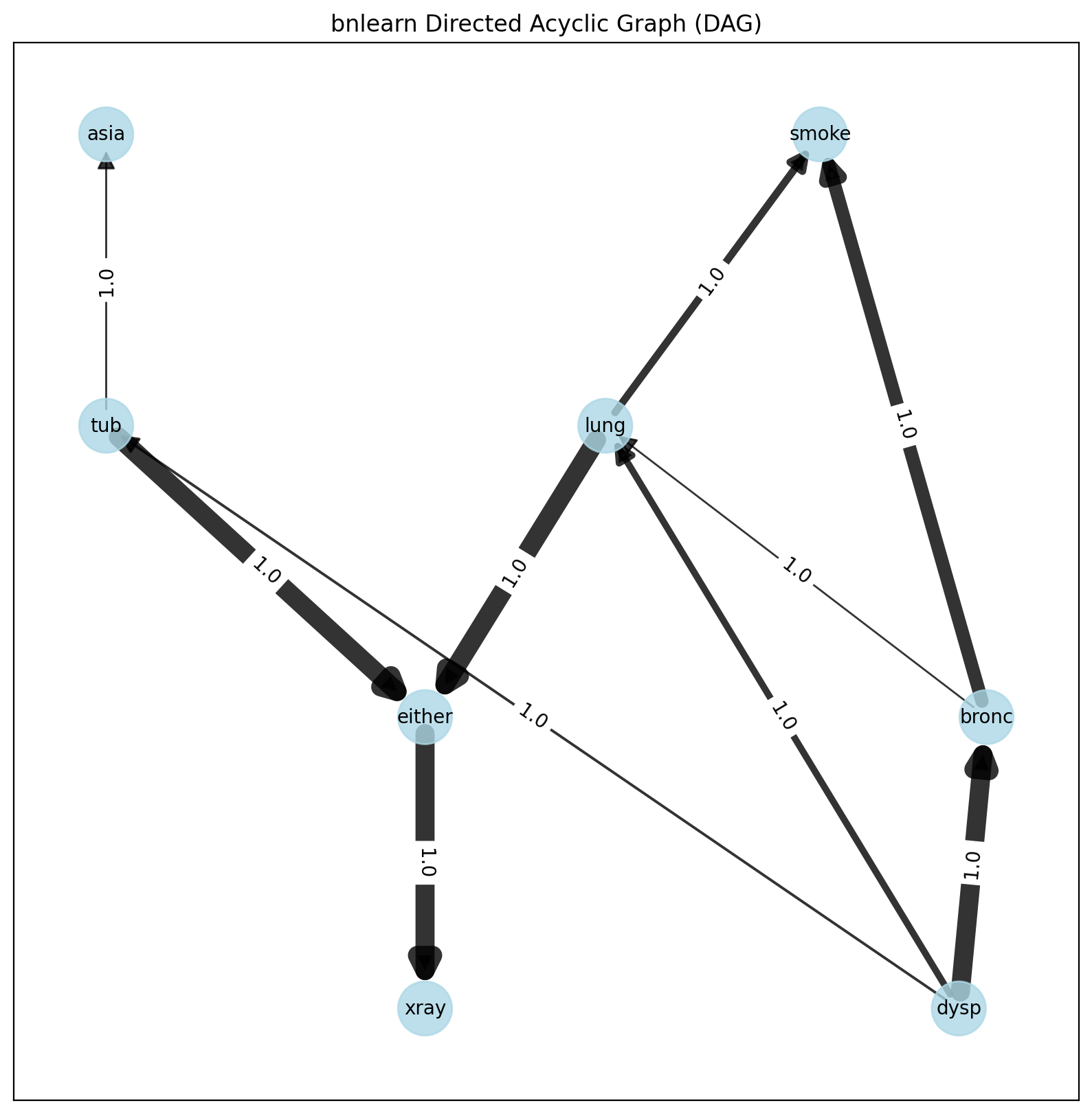
Learned DAG based on dataset.

# Plot based on structure learning of sampled data
bn.plot(model_learned, pos=G['pos'])
# Compare networks and make plot
bn.compare_networks(model_true, model_learned, pos=G['pos'])

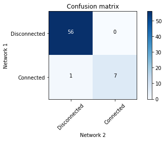
Comparison of True vs. learned DAG.

Parameter Learning Example

Extracting adjacency matrix after Parameter learning:

import bnlearn as bn
# Load dataframe
df = bnlearn.import_example()
# Import DAG
DAG = bnlearn.import_DAG('sprinkler', CPD=False)
# Learn parameters
model = bnlearn.parameter_learning.fit(DAG, df)
# adjacency matrix:
model['adjmat']

# print
print(model['adjmat'])

	Cloudy	Sprinkler	Rain	Wet_Grass
Cloudy	False	True	True	False
Sprinkler	False	False	False	True
Rain	False	False	False	True
Wet_Grass	False	False	False	False

Create a Bayesian Network, learn its parameters from data and perform the inference

Lets make an example were we have data with many measurements, and we have expert information of the relations between nodes. Our goal is to create DAG on the expert knowledge and learn the CPDs. To showcase this, I will use the sprinkler example.

Import example dataset of the sprinkler dataset.

pip install tabulate

import bnlearn as bn
from tabulate import tabulate

df = bn.import_example('sprinkler')
print(tabulate(df.head(), tablefmt="grid", headers="keys"))

	Cloudy	Sprinkler	Rain	Wet_Grass
0	0	0	0	0
1	1	0	1	1
2	0	1	0	1
3	1	1	1	1
4	1	1	1	1
	…	…	…	…

Define the network structure. This can be based on expert knowledge.

edges = [('Cloudy', 'Sprinkler'),
         ('Cloudy', 'Rain'),
         ('Sprinkler', 'Wet_Grass'),
         ('Rain', 'Wet_Grass')]

Make the actual Bayesian DAG

import bnlearn as bn
DAG = bn.make_DAG(edges)
# [BNLEARN] Bayesian DAG created.

# Print the CPDs
CPDs = bn.print_CPD(DAG)
# [BNLEARN.print_CPD] No CPDs to print. Use bnlearn.plot(DAG) to make a plot.

Plot the DAG

bn.plot(DAG)

Parameter learning on the user-defined DAG and input data using maximumlikelihood.

DAG = bn.parameter_learning.fit(DAG, df, methodtype='maximumlikelihood')

Lets print the learned CPDs:

CPDs = bn.print_CPD(DAG)

# [BNLEARN.print_CPD] Independencies:
# (Cloudy _|_ Wet_Grass | Rain, Sprinkler)
# (Sprinkler _|_ Rain | Cloudy)
# (Rain _|_ Sprinkler | Cloudy)
# (Wet_Grass _|_ Cloudy | Rain, Sprinkler)
# [BNLEARN.print_CPD] Nodes: ['Cloudy', 'Sprinkler', 'Rain', 'Wet_Grass']
# [BNLEARN.print_CPD] Edges: [('Cloudy', 'Sprinkler'), ('Cloudy', 'Rain'), ('Sprinkler', 'Wet_Grass'), ('Rain', 'Wet_Grass')]

CPD of Cloudy:

Cloudy(0)	0.494
Cloudy(1)	0.506

CPD of Sprinkler:

Cloudy	Cloudy(0)	Cloudy(1)
Sprinkler(0)	0.4807692307692308	0.7075098814229249
Sprinkler(1)	0.5192307692307693	0.2924901185770751

CPD of Rain:

Cloudy	Cloudy(0)	Cloudy(1)
Rain(0)	0.6518218623481782	0.33695652173913043
Rain(1)	0.3481781376518219	0.6630434782608695

CPD of Wet_Grass:

Rain	Rain(0)	Rain(0)	Rain(1)	Rain(1)
Sprinkler	Sprinkler(0)	Sprinkler(1)	Sprinkler(0)	Sprinkler(1)
Wet_Grass(0)	0.7553816046966731	0.33755274261603374	0.25588235294117645	0.37910447761194027
Wet_Grass(1)	0.2446183953033268	0.6624472573839663	0.7441176470588236	0.6208955223880597

Lets make an inference:

q1 = bn.inference.fit(DAG, variables=['Wet_Grass'], evidence={'Rain':1, 'Sprinkler':0, 'Cloudy':1})

+--------------+------------------+
| Wet_Grass    |   phi(Wet_Grass) |
+==============+==================+
| Wet_Grass(0) |           0.2559 |
+--------------+------------------+
| Wet_Grass(1) |           0.7441 |
+--------------+------------------+

Print the values:

print(q1.df)
# array([0.25588235, 0.74411765])

---

---