Classification Examples
Some of the described examples can also be found in the Colab notebooks: See classification Colab notebook.
xgboost two-class
Function documentation can be found here hgboost.hgboost.hgboost.xgboost()
# Import library
from hgboost import hgboost

# Initialize
hgb = hgboost(max_eval=250, threshold=0.5, cv=5, test_size=0.2, val_size=0.2, top_cv_evals=10, random_state=None, verbose=3)

# Load example data set
df = hgb.import_example()
# Prepare data for classification
y = df['Survived'].values
del df['Survived']
X = hgb.preprocessing(df, verbose=0)

# Fit best model with desired evaluation metric:
results = hgb.xgboost(X, y, pos_label=1, eval_metric='f1')
# [hgboost] >Start hgboost classification..
# [hgboost] >Collecting xgb_clf parameters.
# [hgboost] >Number of variables in search space is [10], loss function: [f1].
# [hgboost] >method: xgb_clf
# [hgboost] >eval_metric: f1
# [hgboost] >greater_is_better: True
# [hgboost] >Total dataset: (891, 204)
# [hgboost] >Hyperparameter optimization..

# Plot the parameter space
hgb.plot_params()
# Plot the summary results
hgb.plot()
# Plot the best performing tree
hgb.treeplot()
# Plot results on the validation set
hgb.plot_validation()
# Plot results on the cross-validation
hgb.plot_cv()

# Make new prdiction using the model (suppose that X is new and unseen data which is similarly prepared as for the learning process)
y_pred, y_proba = hgb.predict(X)
catboost
Function documentation can be found here hgboost.hgboost.hgboost.catboost()
# Import library
from hgboost import hgboost

# Initialize
hgb = hgboost(max_eval=250, threshold=0.5, cv=5, test_size=0.2, val_size=0.2, top_cv_evals=10, random_state=None, verbose=3)

# Load example data set
df = hgb.import_example()
# Prepare data for classification
y = df['Survived'].values
del df['Survived']
X = hgb.preprocessing(df, verbose=0)

# Fit best model with desired evaluation metric:
results = hgb.catboost(X, y, pos_label=1, eval_metric='auc')
# [hgboost] >Start hgboost classification..
# [hgboost] >Collecting ctb_clf parameters.
# [hgboost] >Number of variables in search space is [10], loss function: [auc].
# [hgboost] >method: ctb_clf
# [hgboost] >eval_metric: auc
# [hgboost] >greater_is_better: True
# [hgboost] >Total dataset: (891, 204)
# [hgboost] >Hyperparameter optimization..

# Plot the parameter space
hgb.plot_params()
# Plot the summary results
hgb.plot()
# Plot the best performing tree
hgb.treeplot()
# Plot results on the validation set
hgb.plot_validation()
# Plot results on the cross-validation
hgb.plot_cv()

# Make new prdiction using the model (suppose that X is new and unseen data which is similarly prepared as for the learning process)
y_pred, y_proba = hgb.predict(X)
lightboost
Function documentation can be found here hgboost.hgboost.hgboost.lightboost()
# Import library
from hgboost import hgboost

# Initialize
hgb = hgboost(max_eval=250, threshold=0.5, cv=5, test_size=0.2, val_size=0.2, top_cv_evals=10, random_state=None, verbose=3)

# Load example data set
df = hgb.import_example()
# Prepare data for classification
y = df['Survived'].values
del df['Survived']
X = hgb.preprocessing(df, verbose=0)

# Fit best model with desired evaluation metric:
results = hgb.lightboost(X, y, pos_label=1, eval_metric='auc')
# [hgboost] >Start hgboost classification..
# [hgboost] >Collecting lgb_clf parameters.
# [hgboost] >Number of variables in search space is [10], loss function: [auc].
# [hgboost] >method: lgb_clf
# [hgboost] >eval_metric: auc
# [hgboost] >greater_is_better: True
# [hgboost] >Total dataset: (891, 204)
# [hgboost] >Hyperparameter optimization..

# Plot the parameter space
hgb.plot_params()
# Plot the summary results
hgb.plot()
# Plot the best performing tree
hgb.treeplot()
# Plot results on the validation set
hgb.plot_validation()
# Plot results on the cross-validation
hgb.plot_cv()

# Make new prdiction using the model (suppose that X is new and unseen data which is similarly prepared as for the learning process)
y_pred, y_proba = hgb.predict(X)
Multi-classification Examples
xgboost multi-class
Function documentation can be found here hgboost.hgboost.hgboost.xgboost()
# Import library
from hgboost import hgboost

# Initialize
hgb = hgboost(max_eval=250, threshold=0.5, cv=5, test_size=0.2, val_size=0.2, top_cv_evals=10, random_state=None, verbose=3)

# Load example data set
df = hgb.import_example()
# Prepare data for classification
y = df['Parch'].values
y[y>=3]=3
del df['Parch']
X = hgb.preprocessing(df, verbose=0)

# Fit best model with desired evaluation metric:
results = hgb.xgboost(X, y, method='xgb_clf_multi', eval_metric='kappa')
# [hgboost] >Start hgboost classification..
# [hgboost] >Collecting xgb_clf parameters
# [hgboost] >Number of variables in search space is [10], loss function: [kappa]
# [hgboost] >method: xgb_clf_multi
# [hgboost] >eval_metric: kappa
# [hgboost] >greater_is_better: True
# [hgboost] >Total dataset: (891, 204)
# [hgboost] >Hyperparameter optimization..

# Plot the parameter space
hgb.plot_params()
# Plot the summary results
hgb.plot()
# Plot the best performing tree
hgb.treeplot()
# Plot results on the validation set
hgb.plot_validation()
# Plot results on the cross-validation
hgb.plot_cv()

# Make new prdiction using the model (suppose that X is new and unseen data which is similarly prepared as for the learning process)
y_pred, y_proba = hgb.predict(X)
Regression Examples
Some of the described examples can also be found in the notebooks: See regression Colab notebook.
xgboost_reg
Function documentation can be found here hgboost.hgboost.hgboost.xgboost_reg()
# Import library
from hgboost import hgboost

# Initialize
hgb = hgboost(max_eval=250, threshold=0.5, cv=5, test_size=0.2, val_size=0.2, top_cv_evals=10, random_state=None)

# Load example data set
df = hgb.import_example()
y = df['Age'].values
del df['Age']
I = ~np.isnan(y)
X = hgb.preprocessing(df, verbose=0)
X = X.loc[I,:]
y = y[I]

# Fit best model with desired evaluation metric:
results = hgb.xgboost_reg(X, y, eval_metric='rmse')
# [hgboost] >Start hgboost regression..
# [hgboost] >Collecting xgb_reg parameters.
# [hgboost] >Number of variables in search space is [10], loss function: [rmse].
# [hgboost] >method: xgb_reg
# [hgboost] >eval_metric: rmse
# [hgboost] >greater_is_better: True
# [hgboost] >Total dataset: (891, 204)
# [hgboost] >Hyperparameter optimization..

# Plot the parameter space
hgb.plot_params()
# Plot the summary results
hgb.plot()
# Plot the best performing tree
hgb.treeplot()
# Plot results on the validation set
hgb.plot_validation()
# Plot results on the cross-validation
hgb.plot_cv()

# Make new prdiction using the model (suppose that X is new and unseen data which is similarly prepared as for the learning process)
y_pred, y_proba = hgb.predict(X)
lightboost_reg
Function documentation can be found here hgboost.hgboost.hgboost.lightboost_reg()
# Import library
from hgboost import hgboost

# Initialize
hgb = hgboost(max_eval=250, threshold=0.5, cv=5, test_size=0.2, val_size=0.2, top_cv_evals=10, random_state=None)

# Load example data set
df = hgb.import_example()
y = df['Age'].values
del df['Age']
I = ~np.isnan(y)
X = hgb.preprocessing(df, verbose=0)
X = X.loc[I,:]
y = y[I]

# Fit best model with desired evaluation metric:
results = hgb.lightboost_reg(X, y, eval_metric='rmse')
# [hgboost] >Start hgboost regression..
# [hgboost] >Collecting lgb_reg parameters.
# [hgboost] >Number of variables in search space is [10], loss function: [rmse].
# [hgboost] >method: lgb_reg
# [hgboost] >eval_metric: rmse
# [hgboost] >greater_is_better: True
# [hgboost] >Total dataset: (891, 204)
# [hgboost] >Hyperparameter optimization..

# Plot the parameter space
hgb.plot_params()
# Plot the summary results
hgb.plot()
# Plot the best performing tree
hgb.treeplot()
# Plot results on the validation set
hgb.plot_validation()
# Plot results on the cross-validation
hgb.plot_cv()

# Make new prdiction using the model (suppose that X is new and unseen data which is similarly prepared as for the learning process)
y_pred, y_proba = hgb.predict(X)
catboost_reg
Function documentation can be found here hgboost.hgboost.hgboost.catboost_reg()
# Import library
from hgboost import hgboost

# Initialize
hgb = hgboost(max_eval=250, threshold=0.5, cv=5, test_size=0.2, val_size=0.2, top_cv_evals=10, random_state=None)

# Load example data set
df = hgb.import_example()
y = df['Age'].values
del df['Age']
I = ~np.isnan(y)
X = hgb.preprocessing(df, verbose=0)
X = X.loc[I,:]
y = y[I]

# Fit best model with desired evaluation metric:
results = hgb.catboost_reg(X, y, eval_metric='rmse')
# [hgboost] >Start hgboost regression..
# [hgboost] >Collecting ctb_reg parameters.
# [hgboost] >Number of variables in search space is [10], loss function: [rmse].
# [hgboost] >method: ctb_reg
# [hgboost] >eval_metric: rmse
# [hgboost] >greater_is_better: True
# [hgboost] >Total dataset: (891, 204)
# [hgboost] >Hyperparameter optimization..

# Plot the parameter space
hgb.plot_params()
# Plot the summary results
hgb.plot()
# Plot the best performing tree
hgb.treeplot()
# Plot results on the validation set
hgb.plot_validation()
# Plot results on the cross-validation
hgb.plot_cv()

# Make new prdiction using the model (suppose that X is new and unseen data which is similarly prepared as for the learning process)
y_pred, y_proba = hgb.predict(X)
Ensemble Examples
An ensemble is that each of the fitted models, such as xgboost, lightboost and catboost is even further combined into one function.
The results are usually superior compared to single models. However, the model complexity increases and training time too.
An ensemble can be created for both classification and the regression models.
The function documentation can be found here hgboost.hgboost.hgboost.ensemble()
Ensemble Classification
It can be seen from the results that the ensemble classifier performs superior compared to all indiviudal models.
# Import library
from hgboost import hgboost

# Initialize
hgb = hgboost(max_eval=250, threshold=0.5, cv=5, test_size=0.2, val_size=0.2, top_cv_evals=10, random_state=None, verbose=3)

# Import data
df = hgb.import_example()
y = df['Survived'].values
del df['Survived']
X = hgb.preprocessing(df, verbose=0)

# Fit ensemble model using the three boosting methods. By default these are readily set.
results = hgb.ensemble(X, y, pos_label=1)
# [hgboost] >Create ensemble regression model..
# [hgboost] >...
# [hgboost] >Fit ensemble model with [soft] voting..
# [hgboost] >Evalute [ensemble] model on independent validation dataset (179 samples, 20%)
# [hgboost] >[Ensemble] [auc]: -0.9788 on independent validation dataset
# [hgboost] >[xgb_clf]  [auc]: -0.8434 on independent validation dataset
# [hgboost] >[ctb_clf]  [auc]: -0.8875 on independent validation dataset
# [hgboost] >[lgb_clf]  [auc]: -0.8816 on independent validation dataset

# use the predictor
y_pred, y_proba = hgb.predict(X)

# Plot
hgb.plot_validation()
Ensemble Regression
It can be seen from the results that the ensemble classifier performs superior compared to all indiviudal models.
# Import library
from hgboost import hgboost

# Initialize
hgb = hgboost(max_eval=250, threshold=0.5, cv=5, test_size=0.2, val_size=0.2, top_cv_evals=10, random_state=None)

# Load example data set
df = hgb.import_example()
y = df['Age'].values
del df['Age']
I = ~np.isnan(y)
X = hgb.preprocessing(df, verbose=0)
X = X.loc[I,:]
y = y[I]

# Fit ensemble model using the three boosting methods:
results = hgb.ensemble(X, y, methods=['xgb_reg','ctb_reg','lgb_reg'])
# [hgboost] >Create ensemble regression model..
# [hgboost] >...
# [hgboost] >Evalute [ensemble] model on independent validation dataset (143 samples, 20%).
# [hgboost] >[Ensemble] [rmse]: 64.62 on independent validation dataset
# [hgboost] >[xgb_reg]  [rmse]: 172.2 on independent validation dataset
# [hgboost] >[ctb_reg]  [rmse]: 183 on independent validation dataset
# [hgboost] >[lgb_reg]  [rmse]: 205.9 on independent validation dataset

# Make new prdiction using the model (suppose that X is new and unseen data which is similarly prepared as for the learning process)
y_pred, y_proba = hgb.predict(X)

# Plot
hgb.plot_validation()
Plots
For each model, the following 5 plots can be created:
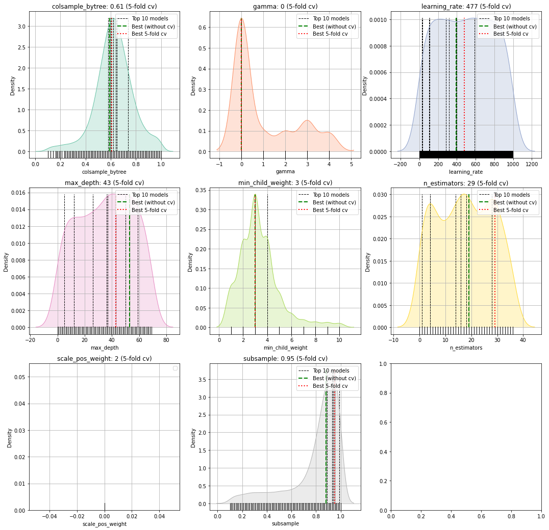
plot_params
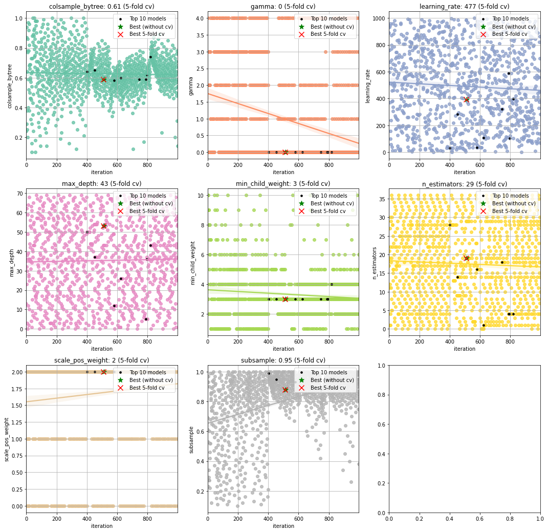
Figure 1 depicts the density of the specific parameter values. As an example, the gamma parameter shows that most iterations converges towards value 0. This may indicate that this parameter with this value has an important role in the in computing the optimal loss. Figure 2 depicts the iterations performed for hyper-optimization per parameter. In case of colsample_bytree we see a convergence towards the range [0.5-0.7].
In both figures, the parameters for all fitted models are plotted together with the best performing models with and without the k-fold crossvalidation. In addition, we also plot the top n performing models. The top performing models can be usefull to deeper examine the used parameter.
Function documentation can be found here hgboost.hgboost.hgboost.plot_params()
# Plot the parameter space
hgb.plot_params()
|
|
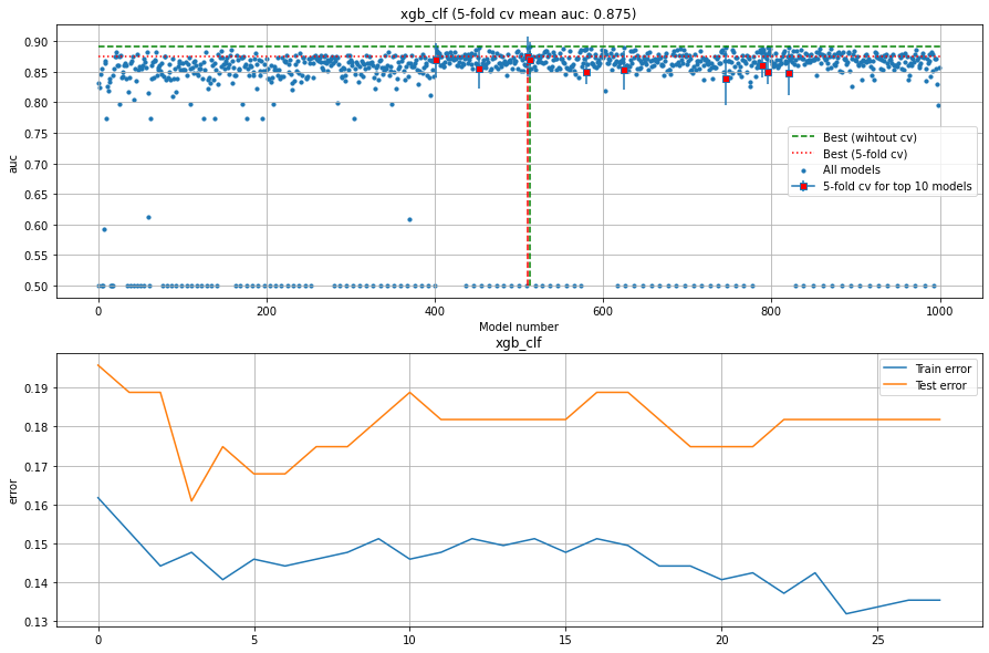
plot summary
This figure exists out of two subfigures. The top figure depicts all evaluated models with the loss score.
The best performing models with and without the k-fold crossvalidation are depicted together with the top n performing models.
The bottom figure depicts the train and test-error.
Function documentation can be found here hgboost.hgboost.hgboost.plot()
# Plot the summary results
hgb.plot()
|
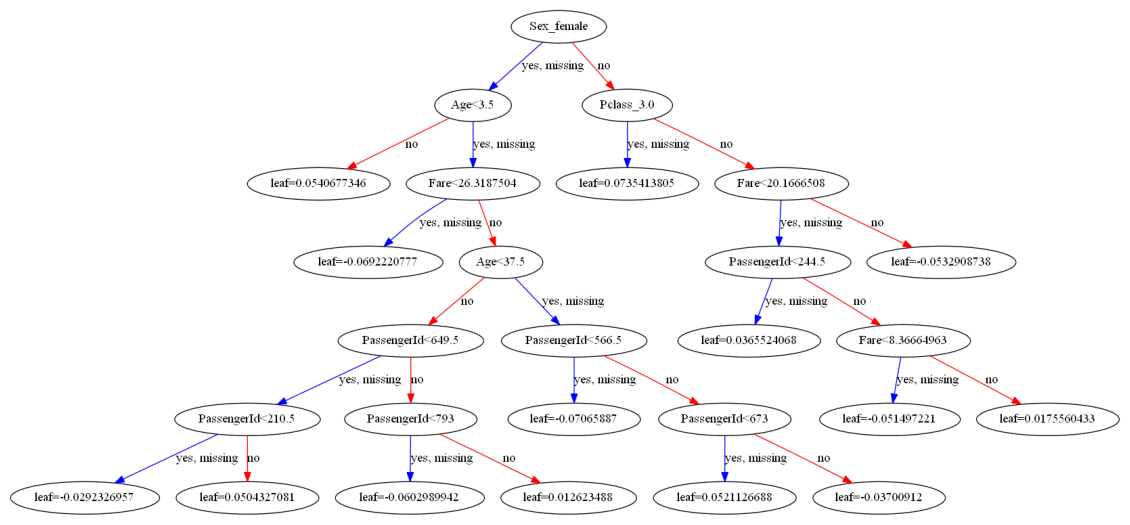
treeplot
Function documentation can be found here hgboost.hgboost.hgboost.treeplot()
# Plot the best performing tree
hgb.treeplot()
|
|
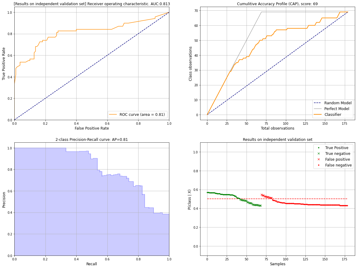
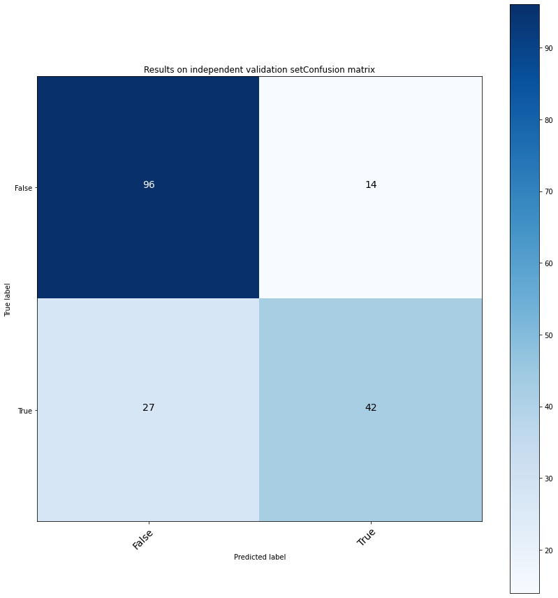
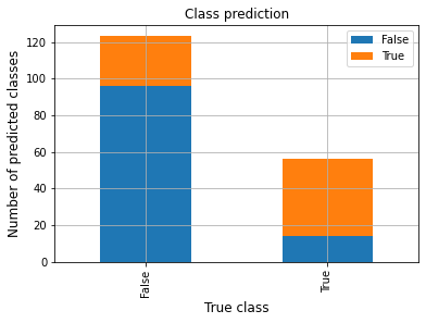
plot_validation
Function documentation can be found here hgboost.hgboost.hgboost.plot_validation()
# Plot results on the validation set
hgb.plot_validation()
|
|
|
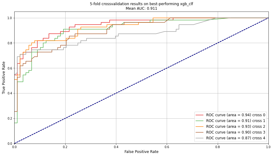
plot_cv
Function documentation can be found here hgboost.hgboost.hgboost.plot_cv()
# Plot results on the cross-validation
hgb.plot_cv()
|