Peakdetect
The peakdetect method [1] is based on the work of Billauer [2] and incorporates improvements from various implementations [3]. This method excels at finding local maxima and minima in noisy signals using findpeaks.peakdetect.peakdetect(), making it particularly valuable for real-world applications where data quality varies.
- Key Advantages:
Noise robustness: Handles noisy data effectively without requiring extensive preprocessing
No smoothing required: Unlike derivative-based methods, it doesn’t require signal smoothing that could lose important peaks
Efficient processing: Optimized for one-dimensional data with configurable parameters
Real-world applicability: Designed for practical signal processing scenarios
The method works exclusively with one-dimensional data and uses a lookahead approach to distinguish between true peaks and noise-induced fluctuations.
One-dimensional data
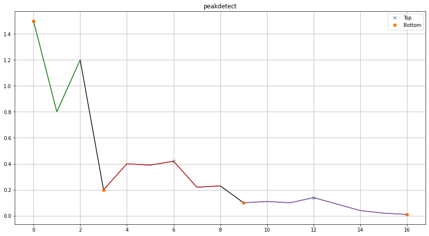
For the peakdetect method, the lookahead parameter is crucial for optimal performance. This parameter defines the distance to look ahead from a peak candidate to determine if it represents a true peak. The default value is 200, but this is typically too large for small datasets (i.e., those with <50 data points).
# Import library
from findpeaks import findpeaks
# Initialize with appropriate lookahead for small dataset
fp = findpeaks(method='peakdetect', lookahead=1, interpolate=None)
# Example 1d-vector
X = fp.import_example('1dpeaks')
# Fit peakdetect method on the 1d-vector
results = fp.fit(X)
# The output contains multiple variables
print(results.keys())
# dict_keys(['df'])

+----+-----+------+--------+----------+--------+
|    |   x |    y |   labx | valley   | peak   |
+====+=====+======+========+==========+========+
|  0 |   0 | 1.5  |      1 | True     | False  |
+----+-----+------+--------+----------+--------+
|  1 |   1 | 0.8  |      1 | False    | False  |
+----+-----+------+--------+----------+--------+
|  2 |   2 | 1.2  |      1 | False    | False  |
+----+-----+------+--------+----------+--------+
|  3 |   3 | 0.2  |      2 | True     | False  |
+----+-----+------+--------+----------+--------+
|  4 |   4 | 0.4  |      2 | False    | False  |
+----+-----+------+--------+----------+--------+
|  5 |   5 | 0.39 |      2 | False    | False  |
+----+-----+------+--------+----------+--------+
|  6 |   6 | 0.42 |      2 | False    | True   |
+----+-----+------+--------+----------+--------+
|  7 |   7 | 0.22 |      2 | False    | False  |
+----+-----+------+--------+----------+--------+
|  8 |   8 | 0.23 |      2 | False    | False  |
+----+-----+------+--------+----------+--------+
|  9 |   9 | 0.1  |      3 | True     | False  |
+----+-----+------+--------+----------+--------+
| 10 |  10 | 0.11 |      3 | False    | False  |
+----+-----+------+--------+----------+--------+
| 11 |  11 | 0.1  |      3 | False    | False  |
+----+-----+------+--------+----------+--------+
| 12 |  12 | 0.14 |      3 | False    | True   |
+----+-----+------+--------+----------+--------+
| 13 |  13 | 0.09 |      3 | False    | False  |
+----+-----+------+--------+----------+--------+
| 14 |  14 | 0.04 |      3 | False    | False  |
+----+-----+------+--------+----------+--------+
| 15 |  15 | 0.02 |      3 | False    | False  |
+----+-----+------+--------+----------+--------+
| 16 |  16 | 0.01 |      3 | True     | False  |
+----+-----+------+--------+----------+--------+
The output is a dictionary containing a single dataframe (df) that provides comprehensive information for follow-up analysis. See: findpeaks.findpeaks.findpeaks.peaks1d()
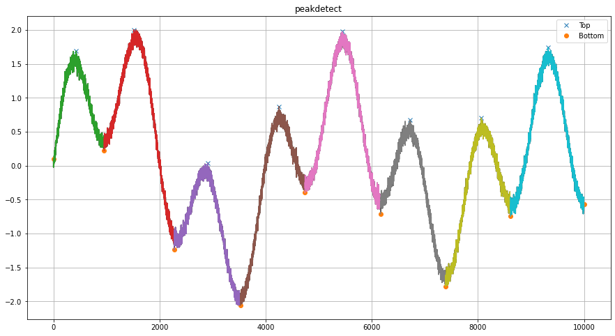
The method’s strength becomes particularly evident when applied to noisy datasets, where it can distinguish between true peaks and noise-induced fluctuations.
# Import library
from findpeaks import findpeaks
# Initialize with appropriate lookahead for large dataset
fp = findpeaks(method='peakdetect', lookahead=200, interpolate=None)

# Example 1d-vector with noise
i = 10000
xs = np.linspace(0,3.7*np.pi,i)
X = (0.3*np.sin(xs) + np.sin(1.3 * xs) + 0.9 * np.sin(4.2 * xs) + 0.06 * np.random.randn(i))

# Fit peakdetect method on the noisy 1d-vector
results = fp.fit(X)
# Plot
fp.plot()