Multivariate Parameter Fitting
The distfit library provides multivariate distribution fitting that enables modeling complex dependencies between multiple variables using copula-based methods.
Rather than assuming a single multivariate parametric distribution, distfit decomposes the problem into:
Univariate marginal distribution fitting
Dependence modeling via a Gaussian copula
This separation allows flexible modeling of heterogeneous marginals while still capturing multivariate structure.
Core Features
Multivariate distribution fitting with automatic marginal estimation
Gaussian copula–based dependence modeling
Joint density evaluation for relative likelihood comparison
Multivariate outlier detection using joint log-density
Synthetic data generation preserving marginals and dependence
Extensive visualization tools for copula diagnostics
Marginal Distribution Fitting
Each variable is fitted independently using univariate distributions. You need to set multivariate=True and you can also set all other parameters as desired.
dfit = distfit(
    multivariate=True,
    distr='norm',
    method='mle',
    bins=50,
    alpha=0.05
)
Copula Dependence Modeling
Dependence is modeled using a Gaussian copula, where \(\Sigma\) is the estimated correlation matrix.
Joint Density Evaluation
The joint density is computed as:
with copula density:
Quick Example for Multivariate Fitting
from distfit import distfit

# Initialize with multivariate mode
dfit = distfit(multivariate=True)

# Load example data
X = dfit.import_example(data='multi_normal')
# X = dfit.import_example(data='multi_t')

# Fit model
dfit.fit_transform(X)

# Access estimated correlation matrix (Gaussian copula)
print(dfit.model.corr)

# Evaluate joint density
results = dfit.evaluate_pdf(X)
print(results['score'])
print(results['copula_density'])

# Generate synthetic samples
Xnew = dfit.generate(n=10)

# Detect multivariate outliers
bool_outliers = dfit.predict_outliers(X)
Interpretation output
results = dfit.evaluate_pdf(X)

# Output
results['copula_density']
results['score']
copula_densityVector of joint density values, one per observation. These are relative likelihoods, not probabilities.scoreMean log joint density, where higher values indicate a better model fit when comparing models on the same data.\[\text{score} = \frac{1}{n} \sum_{i=1}^{n} \log f(\mathbf{x}_i)\]
Plots
Copula Gaussian Density
This visualization shows the data transformed to Gaussian copula space, where \(F_i\) are fitted marginal CDFs and \(\Phi^{-1}\) is the inverse standard normal CDF.
- Interpretation
Each point represents an observation in latent Gaussian space
Elliptical contours indicate linear dependence
Structure reflects dependence only, not marginal shape
fig, ax = dfit.plot_copulaDensity(plot_type='gaussian', pairplot=False)
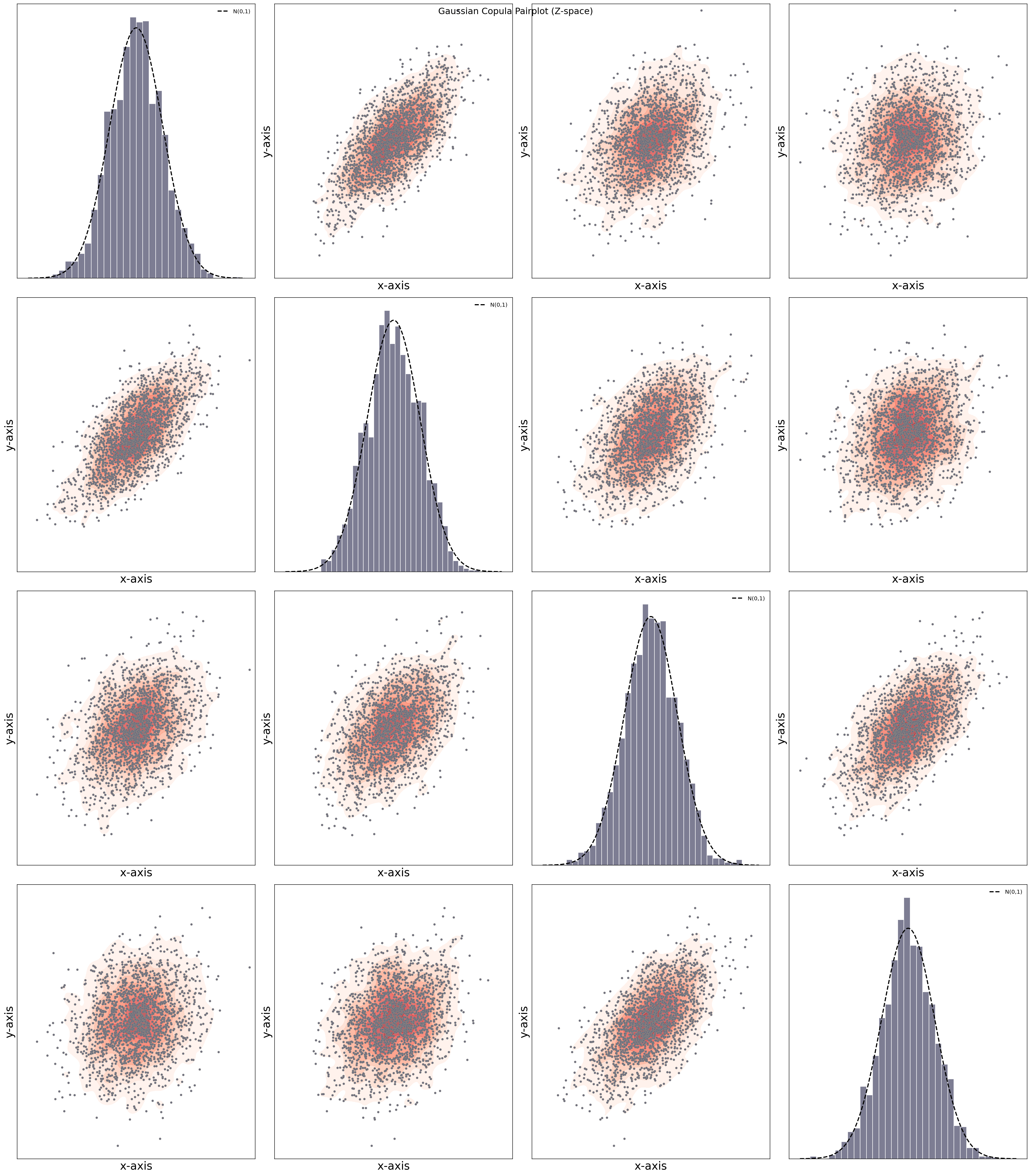
Copula Gaussian Density Pairplot
- Interpretation
Diagonal panels show marginal distributions in Gaussian space
Off-diagonal panels show pairwise dependence
Linear structure indicates strong dependence
Circular scatter indicates weak or no dependence
fig, ax = dfit.plot_copulaDensity(plot_type='gaussian', pairplot=True)
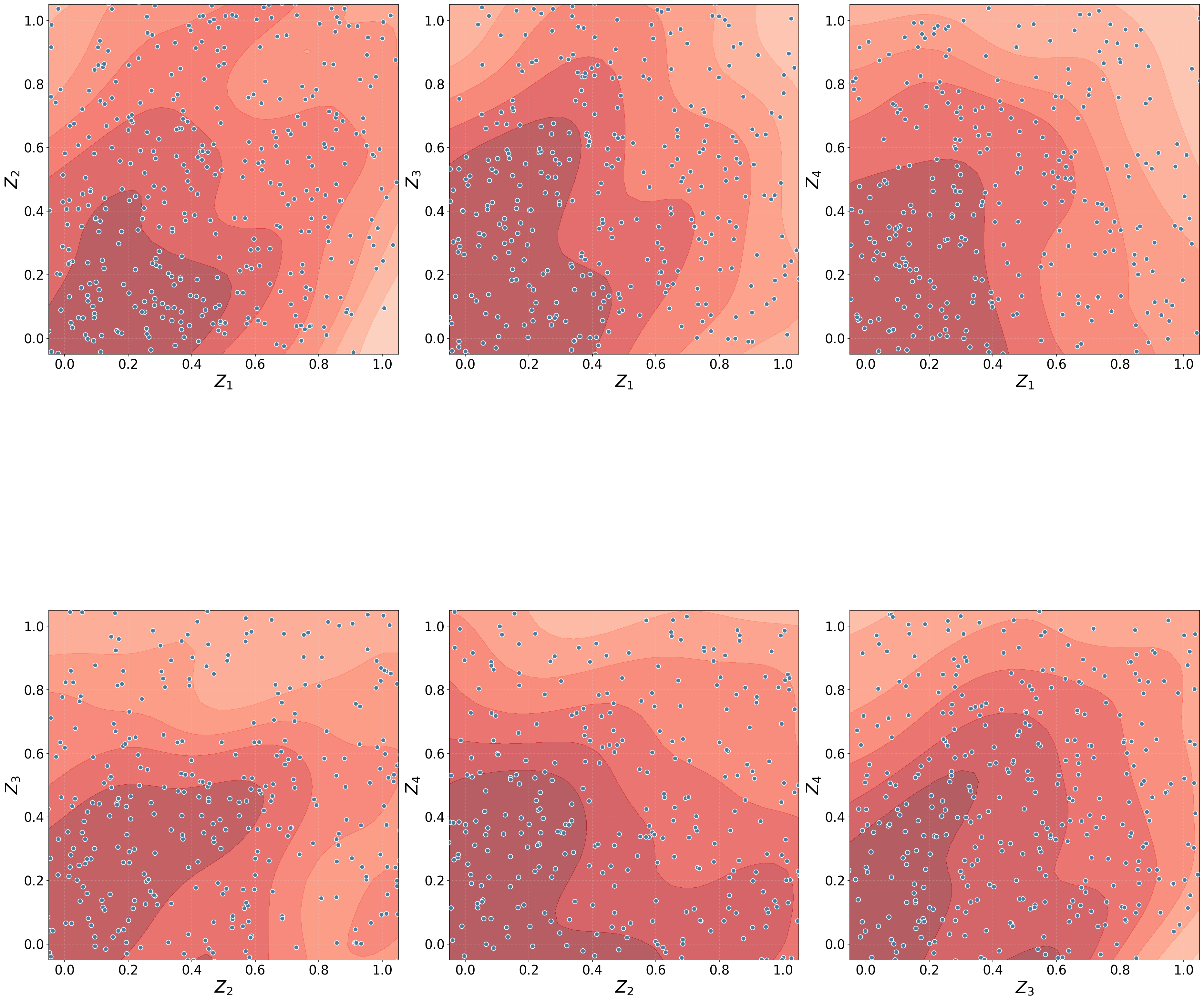
Copula Uniform Density
This visualization shows the data in copula (uniform) space.
- Interpretation
All marginals are uniform on \([0,1]\)
Structure reflects dependence only
Uniform scatter implies independence
Clustering near corners suggests tail dependence
fig, ax = dfit.plot_copulaDensity(plot_type='uniform', pairplot=False)
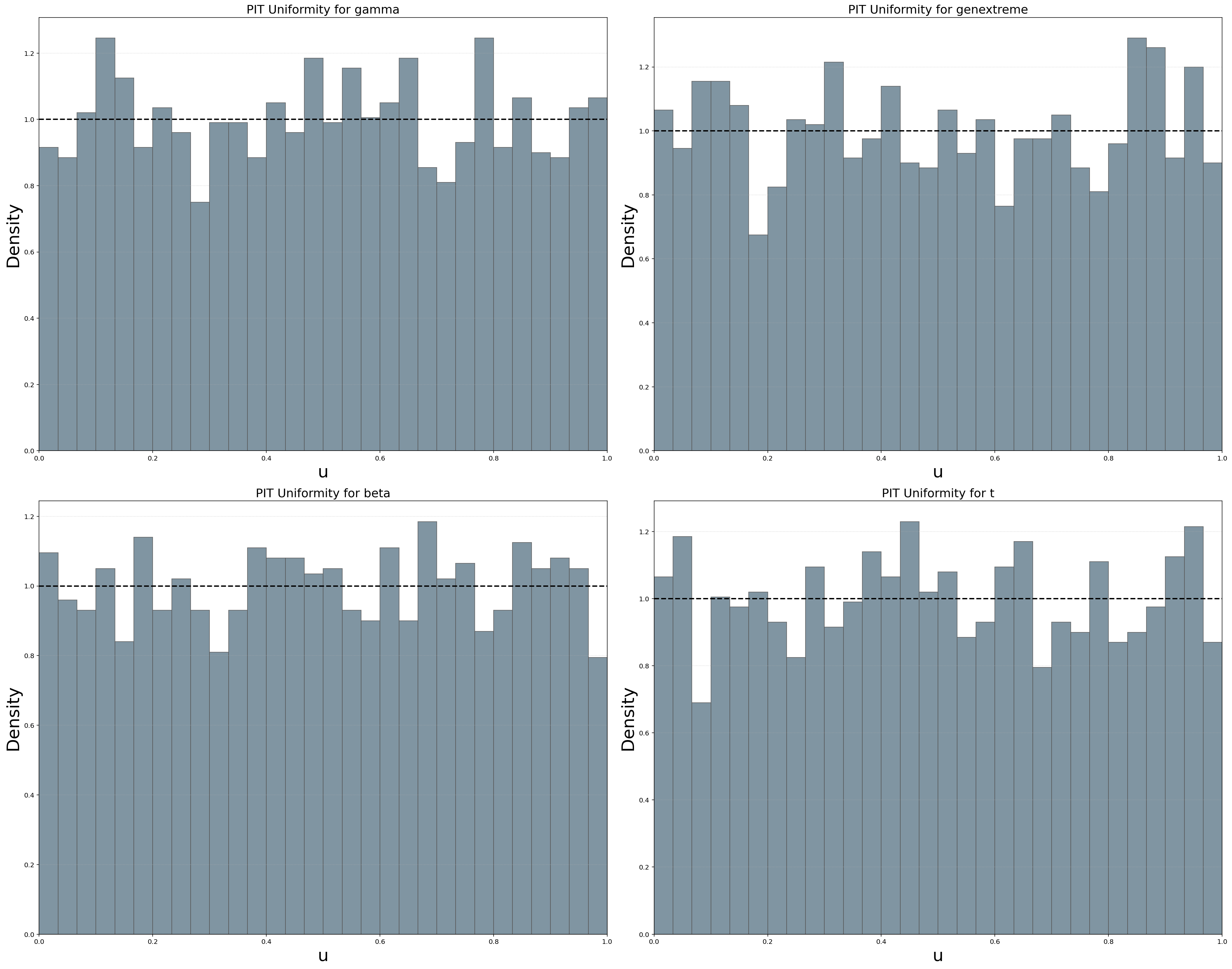

Copula Uniform Density Pairplot
- Interpretation
Diagonal panels test PIT uniformity
Off-diagonal panels show empirical copula structure
Deviations indicate marginal misfit or dependence
fig, ax = dfit.plot_copulaDensity(plot_type='uniform', pairplot=True)

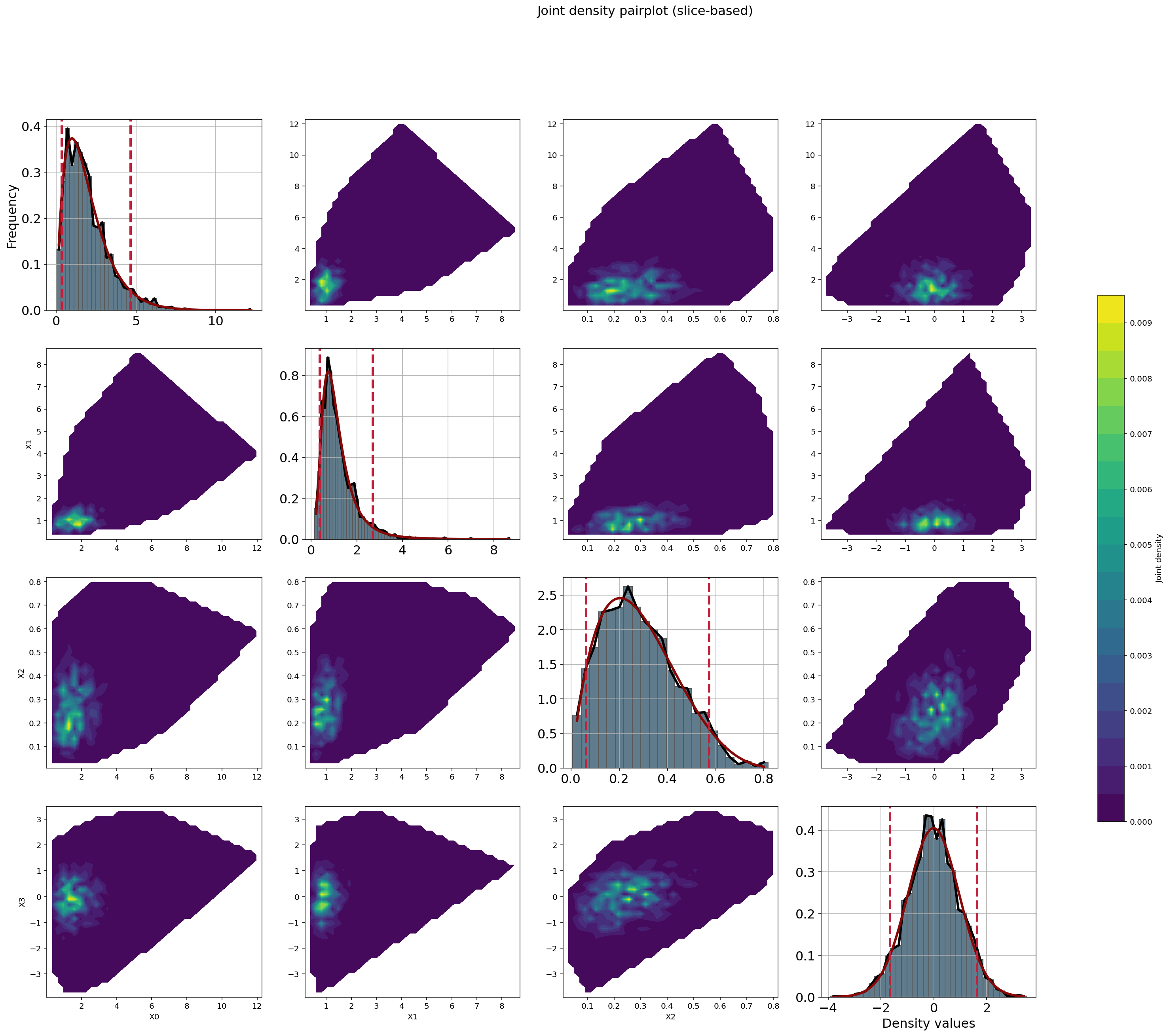
Joint Density Plot
- Interpretation
Displays bivariate slices of the joint density
Combines marginal distributions and dependence
Higher dimensions are visualized via pairwise projections
fig, ax = dfit.plot_jointDensity(X)
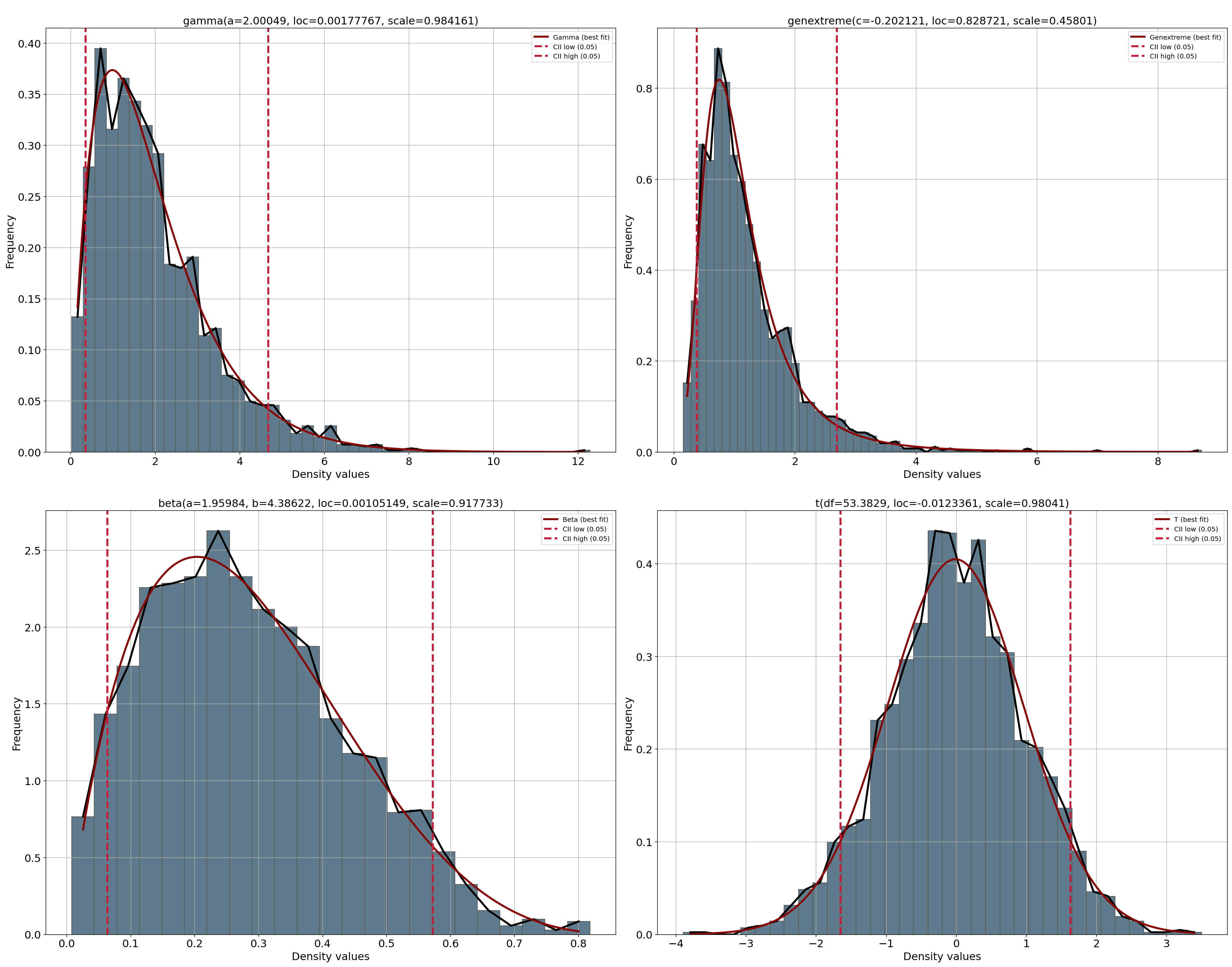
PDF Plot
- Interpretation
Shows fitted marginal probability density functions
Used to assess marginal distribution fit
fig, ax = dfit.plot(chart='pdf')
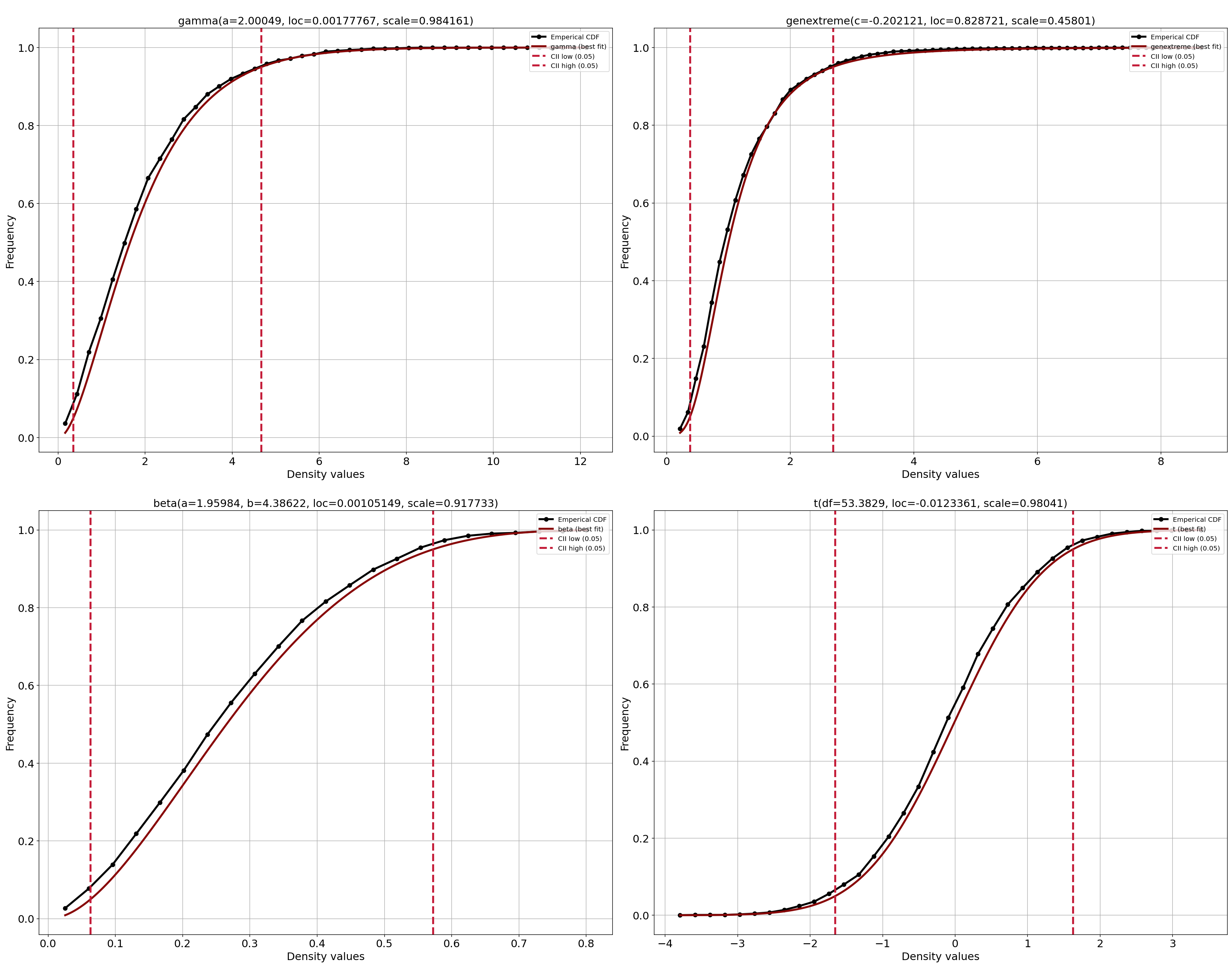
CDF Plot
- Interpretation
Shows fitted marginal cumulative distribution functions
Used to validate probability integral transforms
fig, ax = dfit.plot(chart='cdf')
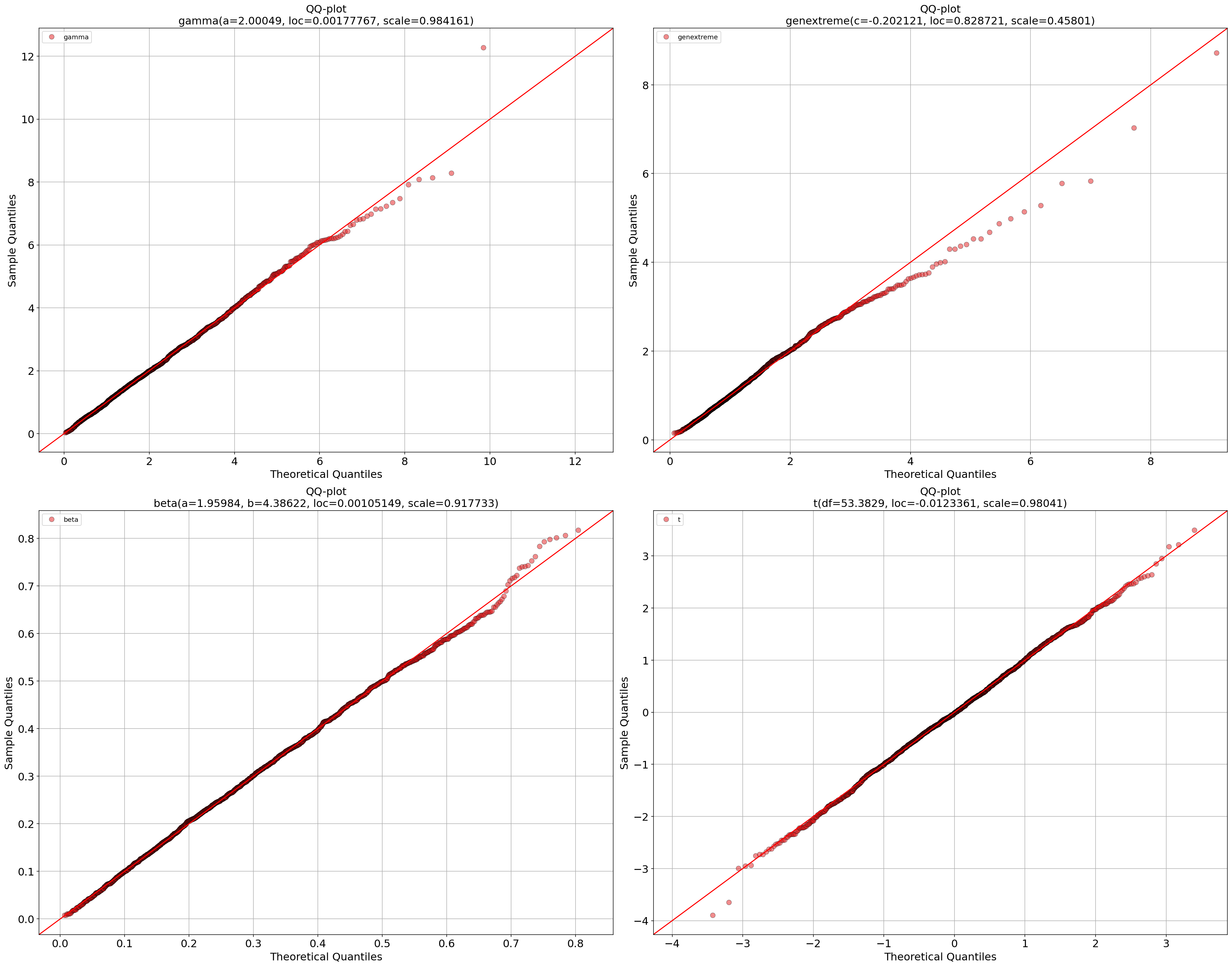
QQ Plot (Multivariate)
- Interpretation
Compares empirical quantiles to fitted marginals
Large deviations indicate poor marginal fit
Multivariate outliers often appear at extremes
fig, ax = dfit.qqplot(X)
Outlier Detection
Outliers are defined as observations with low joint log-density. This detects observations unlikely under the full multivariate model, even if they are not marginal outliers.
outliers = dfit.predict_outliers(X)
It is expected that outliers have lower likelihood. We can expect that as shown in the code-block.
rng = np.random.default_rng(42)
mean = [0, 0]
cov = [[1, 0.6],
       [0.6, 1]]

X = rng.multivariate_normal(mean, cov, size=2000)

# Fit model on multivariate normal random data
dfit = distfit(multivariate=True, verbose=False)
dfit.fit_transform(X)

# Evaluate the copula density
pdf = dfit.evaluate_pdf(X)["copula_density"]

# Get outliers
outliers = dfit.predict_outliers(X)

# Outliers have lower likelihood
print(np.mean(pdf[outliers]))
# 0.0014758104978686533

print(np.mean(pdf[~outliers]))
# 0.10025029900211244

print(np.mean(pdf[outliers]) < np.mean(pdf[~outliers]))
# True
Generate Synthetic Data
Generate multivariate synthetic data based on the multidistribution fit.
# Generate synthetic samples
Xnew = dfit.generate(n=10)

 array([[ 0.61334212,  0.55326009,  0.15892912, -0.08668606],
     [ 1.12584863,  1.14758074,  0.18494332, -0.80220606],
     [ 3.72283115,  0.62819404,  0.31963464, -0.13226541],
     [ 1.05816854,  0.52648982,  0.30748156, -0.10778112],
     [ 0.48590115,  0.5370091 ,  0.31400217,  0.08802375],
     [ 0.51329513,  0.34469918,  0.12943172,  0.74397221],
     [ 1.3917044 ,  1.17482342,  0.30421591, -0.09497158],
     [ 0.42975052,  0.6232065 ,  0.25283493, -0.31761824],
     [ 0.27751107,  0.5779773 ,  0.35859482,  1.66407101],
     [ 1.13505836,  0.41056057,  0.24425488, -0.18984279]])
Model Comparison
Use the mean log-density score for comparison. Higher scores indicate better fit (for the same data).
res1 = model1.evaluate_pdf(X)
res2 = model2.evaluate_pdf(X)

print(res1['score'], res2['score'])
Connected variables
In a Gaussian copula model, all dependencies between variables are encoded in the
correlation matrix stored in dfit.model.corr. Each entry
corr[i, j] represents the linear dependence between variable i and j in
Gaussian copula space.
- This correlation matrix induces a graph structure where:
Nodes correspond to variables (columns of
X)Edges exist when two variables have a non-zero (or sufficiently large) correlation
By analysing this graph, we can identify connected components: groups of variables that are mutually dependent (directly or indirectly). Variables belonging to different components are statistically independent under the copula model.
- Identifying connected variables helps to:
Interpret the dependency structure learned by the model
Detect independent sub-copulas in high-dimensional data
Explain block-diagonal or near block-diagonal correlation matrices
Simplify diagnostics and model validation
The example below extracts connected components directly from
dfit.model.corr using a depth-first search (DFS). A small threshold can be used to avoid spurious connections caused by numerical noise.
print(dfit.model.corr)

[[1.         0.57622997]
[0.57622997 1.        ]]

# Connected variables for the first variable
dfit.model.corr[:, 0] > 0.8
Caveats and Considerations
Gaussian copula assumes elliptical dependence
Tail dependence may be underestimated
Computational cost increases with dimensionality
Density values are relative likelihoods, not probabilities
Covariance regularization is applied for numerical stability
References
The Gaussian copula relies on the multivariate normal distribution [1] [2].