Discrete Distributions
The method discrete computes the best fit using the binomial distribution when using discrete integer data. The questions can be summarized as following: given a list of nonnegative integers, can we fit a probability distribution for a discrete distribution, and compare the quality of the fit? For discrete quantities, the correct term is probability mass function: P(k) is the probability that a number picked is exactly equal to the integer value k. As far as discrete distributions go, the PMF for one list of integers is of the form P(k) and can only be fitted to the binomial distribution, with suitable values for n and p.
Note that if the best fit is obtained for n=1, then it is a Bernoulli distribution. In addition, for sufficiently large n, a binomial distribution and a Gaussian will appear similar according to B(k, p, n) = G(x=k, mu=p*n, sigma=sqrt(p*(1-p)*n)).
With distfit you can also easily fit a Gaussian distribution if desired.
Binomial Distribution (Discrete)
In order to find the optimal integer n value, you need to vary n, fit p for each n, and pick the n, p combination with the best fit. In the implementation, I estimate n and p from the relation with the mean and sigma value above and search around that value. In principle, the most best fit will be obtained if you set weighted=True (default). However, different evaluation metrics may require setting weighted=False.
It turns out that it is difficult to fit a binomial distribution unless you have a lot of data. Typically, with 500 samples, you get a fit that looks OK by eye, but which does not recover the actual n and p values correctly, although the product n*p is quite accurate. In those cases, the SSE curve has a broad minimum, which is a giveaway that there are several reasonable fits.
Generate Random Discrete Data
Lets see how the fitting works. For this example, I will generate some random numbers:
# Generate random numbers
from scipy.stats import binom
# Set parameters for the test-case
n = 8
p = 0.5

# Generate 10000 samples of the distribution of (n, p)
X = binom(n, p).rvs(10000)
print(X)

# [5 1 4 5 5 6 2 4 6 5 4 4 4 7 3 4 4 2 3 3 4 4 5 1 3 2 7 4 5 2 3 4 3 3 2 3 5
#  4 6 7 6 2 4 3 3 5 3 5 3 4 4 4 7 5 4 5 3 4 3 3 4 3 3 6 3 3 5 4 4 2 3 2 5 7
#  5 4 8 3 4 3 5 4 3 5 5 2 5 6 7 4 5 5 5 4 4 3 4 5 6 2...]
Fit Discrete Model
Initialize distfit for discrete distribution for which the binomial distribution is used. Now we want to fit data X, and determine whether we can retrieve best n and p.
# Import distfit
from distfit import distfit

# Initialize for discrete distribution fitting
dfit = distfit(method='discrete')

# Run distfit to and determine whether we can find the parameters from the data.
dfit.fit_transform(X)

# [distfit] >fit..
# [distfit] >transform..
# [distfit] >Fit using binomial distribution..
# [distfit] >[binomial] [SSE: 7.79] [n: 8] [p: 0.499959] [chi^2: 1.11]
# [distfit] >Compute confidence interval [discrete]

# Get the model and best fitted parameters.
print(dfit.model)

# {'model': <scipy.stats._distn_infrastructure.rv_frozen at 0x1ff23e3beb0>,
#  'params': (8, 0.4999585504197037),
#  'name': 'binom',
#  'SSE': 7.786589839641551,
#  'chi2r': 1.1123699770916502,
#  'n': 8,
#  'p': 0.4999585504197037,
#  'CII_min_alpha': 2.0,
#  'CII_max_alpha': 6.0}

# Best fitted n=8 and p=0.4999 which is great because the input was n=8 and p=0.5
dfit.model['n']
dfit.model['p']
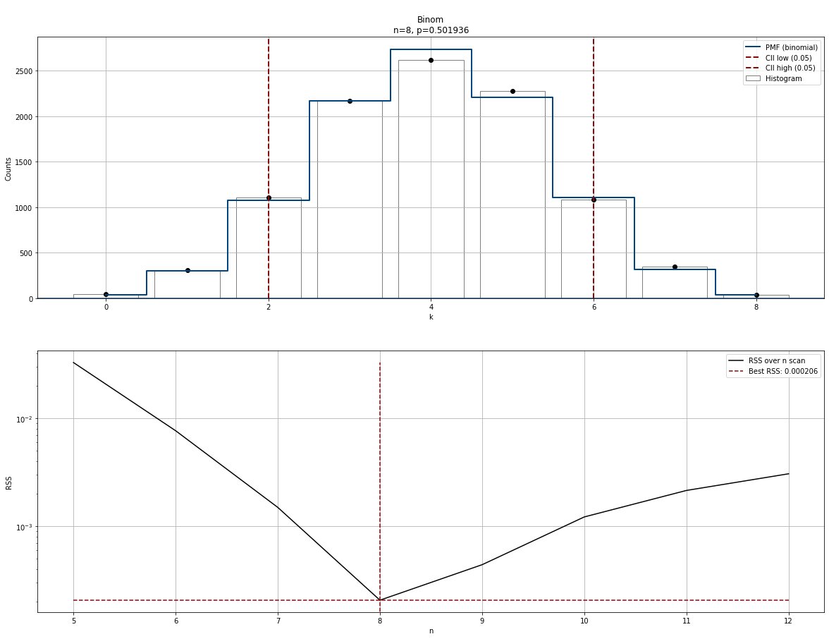
Plot
# Make plot
dfit.plot()
|
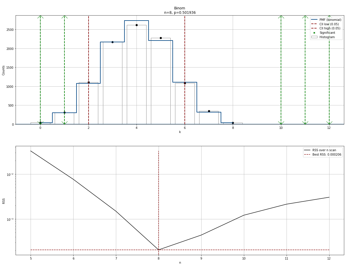
Make predictions
With the fitted model we can start making predictions on new unseen data. Note that P stands for the RAW P-values and y_proba are the corrected P-values after multiple test correction (default: fdr_bh). Final decisions are made on y_proba. In case you want to use the P values, set multtest to None during initialization.
# Some data points for which we want to examine their significance.
y = [0, 1, 10, 11, 12]
results = dfit.predict(y)
dfit.plot()

# Make plot with the results
dfit.plot()

df_results = pd.DataFrame(pd.DataFrame(results))

#   y   y_proba    y_pred   P
#   0   0.004886   down     0.003909
#   1   0.035174   down     0.035174
#   10  0.000000     up     0.000000
#   11  0.000000     up     0.000000
#   12  0.000000     up     0.000000
|
References
Some parts of the binomial fitting is authored by Han-Kwang Nienhuys (2020); copying: CC-BY-SA.