Parameter fitting
The performance of distfit can be examined by various aspects. In this section we will evaluate the detected parameters, and the goodness of fit of the detected probability density function (pdf).
Lets evaluate the performance of distfit of the detected parameters when we draw random samples from a normal (Gaussian) distribution with mu*=0 and *std*=2. We would expect to find *mu and std very close to the input values.
from distfit import distfit
import numpy as np
# Initialize model and specify distribution to be normal
X = np.random.normal(0, 2, 5000)
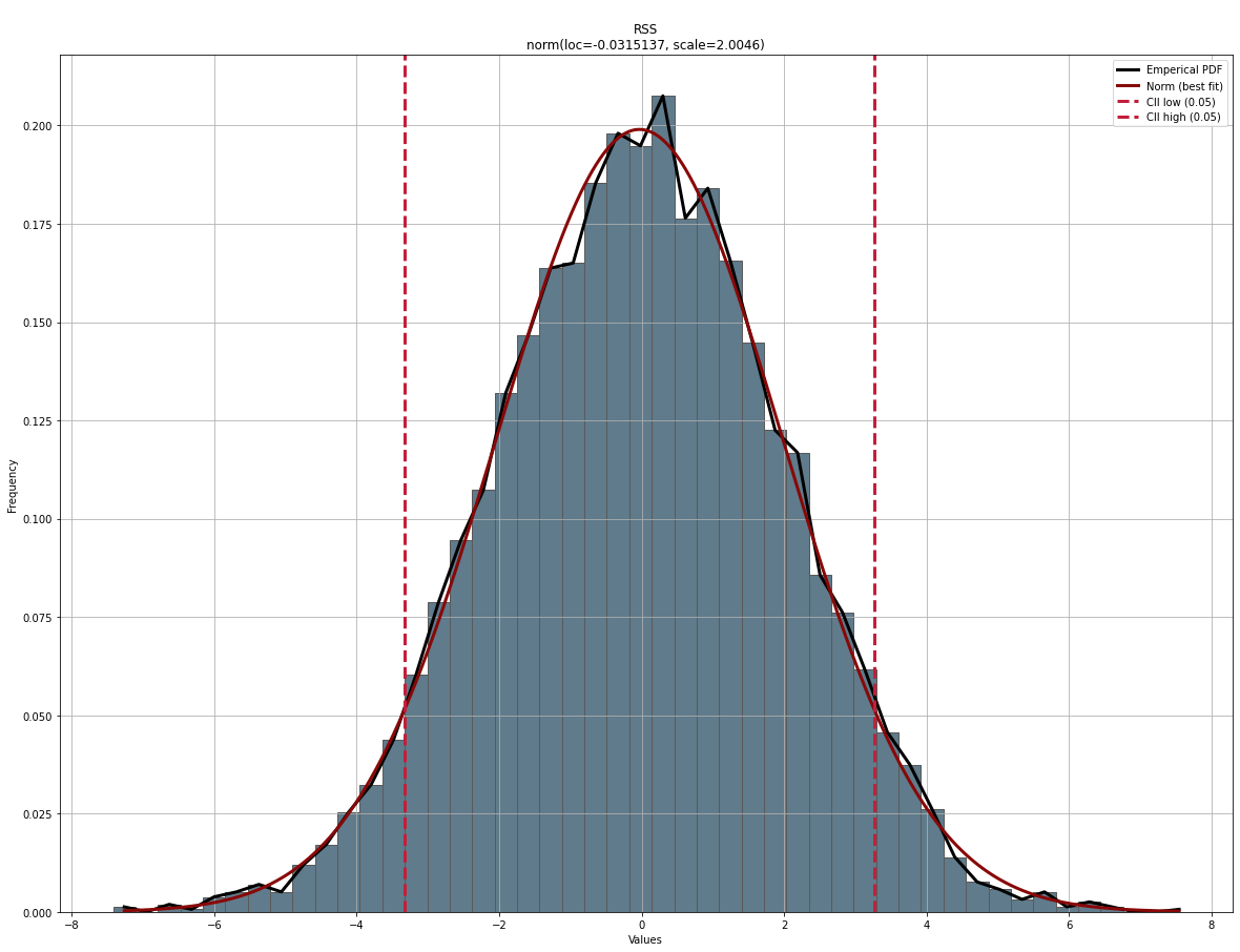
For demonstration puprposes we pre-specify the normal distribution to find the best parameters. When we do that, as shown below, a mean or loc of 0.004 is detected and a standard deviation (scale) with 2.02 which is very close to our input parameters.
dfit = distfit(distr='norm')
dfit.fit_transform(X)
print(dfit.model)

# {'name': 'norm',
#  'score': 0.0008652960233748114,
#  'loc': -0.03151369033439687,
#  'scale': 2.0045971659158206,
#  'arg': (),
#  'params': (-0.03151369033439687, 2.0045971659158206),
#  'model': <scipy.stats._distn_infrastructure.rv_continuous_frozen at 0x1dbd0819450>,
#  'bootstrap_score': 0,
#  'bootstrap_pass': None,
#  'color': '#e41a1c',
#  'CII_min_alpha': -3.3287826092676776,
#  'CII_max_alpha': 3.265755228598883}
dfit.plot(chart='pdf')
Probability Density Function fitting
To measure the goodness of fit of PDFs, we will evaluate multiple PDFs using RSS. The goodness of fit scores are stored in dfit.summary. In this example, we will not specify any distribution but only provide the empirical data and compute the fits for the different PDFs.
An example of the results are shown in the code section.
dfit = distfit()
dfit.fit_transform(X)
print(dfit.summary)

#   distr         score  ...        scale                                     arg
# 0        norm  0.00215419  ...        2.021                                      ()
# 1           t  0.00215429  ...      2.02105                    (2734197.302263666,)
# 2       gamma  0.00216592  ...   0.00599666                   (113584.76147029496,)
# 3        beta  0.00220002  ...      39.4803  (46.39522231565038, 47.98055489856441)
# 4     lognorm  0.00226011  ...      139.173                 (0.014515926633415211,)
# 5  genextreme  0.00370334  ...      2.01326                   (0.2516817342848604,)
# 6    dweibull  0.00617939  ...        1.732                   (1.2681369071313497,)
# 7     uniform    0.244839  ...      14.3579                                      ()
# 8      pareto    0.358765  ...  2.40844e+08                   (31772216.567824945,)
# 9       expon    0.360553  ...      7.51848                                      ()
If we repeat the experiment again, teh results will change slightly due to the stochastic element. See figure below.
dfit.plot_summary()
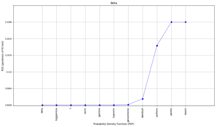
The model detected beta as the best PDF but a good RSS score is also detected for other distributions.
But why did the normal distribution not have the lowest Residual Sum of Squares despite we generated random normal data?
Well, first of all, our input data set will always be a finite list that is bound within a (narrow) range. In contradition, the theoretical (normal) distribution goes to infinity in both directions.
Secondly, all statistical analyses are based on models, and all models are merely simplifications of the real world. Or in other words, to approximate the theoretical distributions, we need to use multiple statistical tests, each with its own (dis)advantages.
Finally, some distributions have a very flexible character for which the (log)gamma is a clear example. For a large k, the gamma distribution converges to normal distribution.
The result is that the top 7 distributions have a similar and low RSS score, among them the normal distribution. We can see in the summary statistics that the estimated parameters for the normal distribution are loc=~0 and scale=~2, which is very close to our initially generated random sample population (mean=0, std=2). All things considered, A very good result.
Bootstrapping
We can further validate our fitted model using a bootstrapping approach and the Kolmogorov-Smirnov (KS) test to assess the goodness of fit. If the model is overfitting, the KS test will reveal a significant difference between the bootstrapped samples and the original data, indicating that the model is not representative of the underlying distribution. In distfit, the n_bootst parameter can be set during initialization or afterward (see code section). Note that bootstrapping is computationally intensive.
The goal here is to estimate the KS statistic of the fitted distribution when the params are estimated from data.
Resample using fitted distribution.
Use the resampled data to fit the distribution.
Compare the resampled data vs. fitted PDF.
Repeat 1000 times the steps 1-3
return score=ratio succes / n_boots
return whether the 95% CII for the KS-test statistic is valid.
# Import library
from distfit import distfit

# Initialize with 100 permutations
dfit = distfit(n_boots=100)

# Generate data from PDF
# X = np.random.exponential(0.5, 10000)
# X = np.random.uniform(0, 1000, 10000)
X = np.random.normal(163, 10, 10000)

# Fit model
results = dfit.fit_transform(X)

# Results are stored in summary
dfit.summary[['name', 'score', 'bootstrap_score', 'bootstrap_pass']]

# Create summary plot
dfit.plot_summary()
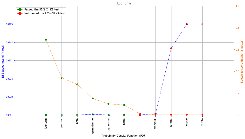
The plot contains on the left axes the goodness of fit test and on the right axes (orange line) the bootstrap result. The bootstrap score is a value between [0, 1] and depicts the fit-success ratio for the number of bootstraps and the PDF. In addition, the green and red dots depict whether there was a significant difference between the bootstrapped samples and the original data. The bootstrap test now excludes a few more PDFs that showed no stable results. The combined information demonstrates that the top 6 distributions are stable, whereas the t-distribution and the dweibull-distribution are not representative for the Emperical data.
Varying sample sizes
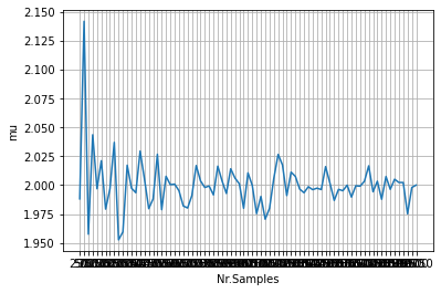
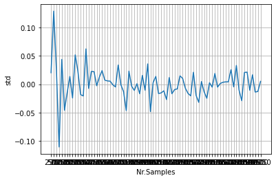
The goodness of fit will change according the number of samples that is provided. In the example above we specified 5000 samples which gave good results. However, with a relative low number of samples, a poor fit can occur. For demonstration purposes we will vary the number of samples and store the mu, std. In this experiment we are generating random continuous values from a normal distribution. We will fixate fitting normal distribution and examine the loc, and scale parameters.
# Initialize without verbose.
dfit = distfit(verbose=0)

# Create random data with varying number of samples
samples = np.arange(250, 10000, 250)

# Initialize model
distr='norm'

# Estimate parameters for the number of samples
for s in samples:
    print(s)
    X = np.random.normal(0, 2, s)
    dfit.fit_transform(X)
    out.append([dfit.model['loc'], dfit.model['scale'], dfit.model['name'], s])
When we plot the results, distfit nicely shows that by increasing the number of samples results in a better fit of the parameters. A convergence towards mu=2 and std=0 is clearly seen.
|
|
Smoothing
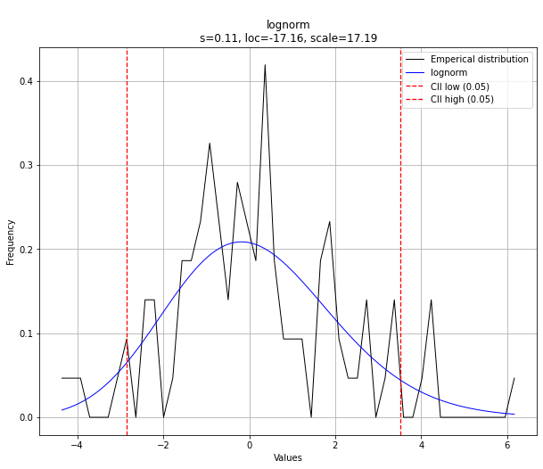
If the number of samples is very low, it can be difficult to get a good fit on your data.
A solution is to play with the bin size, eg. increase bin size.
Another manner is by smoothing the histogram with the smooth parameter. The default is set to None.
Lets evaluate the effect of this parameter.
# Generate data
X = np.random.normal(0, 2, 100)
# Fit model without smoothing
model = distfit()
model.fit_transform(X)
model.plot()

# Fit model with heavy smoothing
model = distfit(smooth=10)
model.fit_transform(X)
model.plot()
|
|
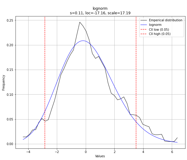
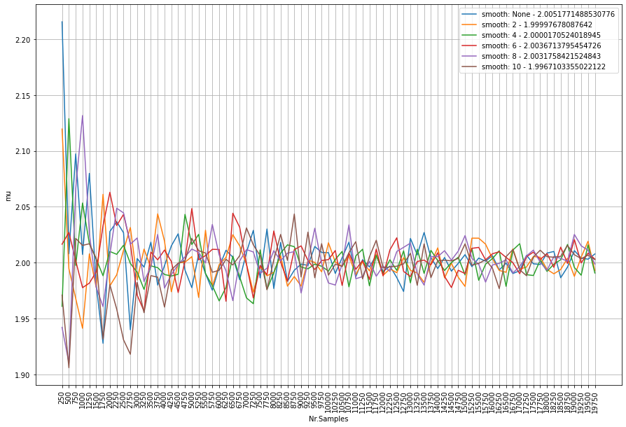
Here we are going to combine the number of samples with the smoothing parameter. It is interesting to see that there is no clear contribution of the smoothing. The legends depicts the smoothing window with the average mu. We see that all smooting windows jump up-and-down the mu=2. However, the more samples, the smaller the variation becomes. The smooting parameter seems to be only effective in very low sample sizes.
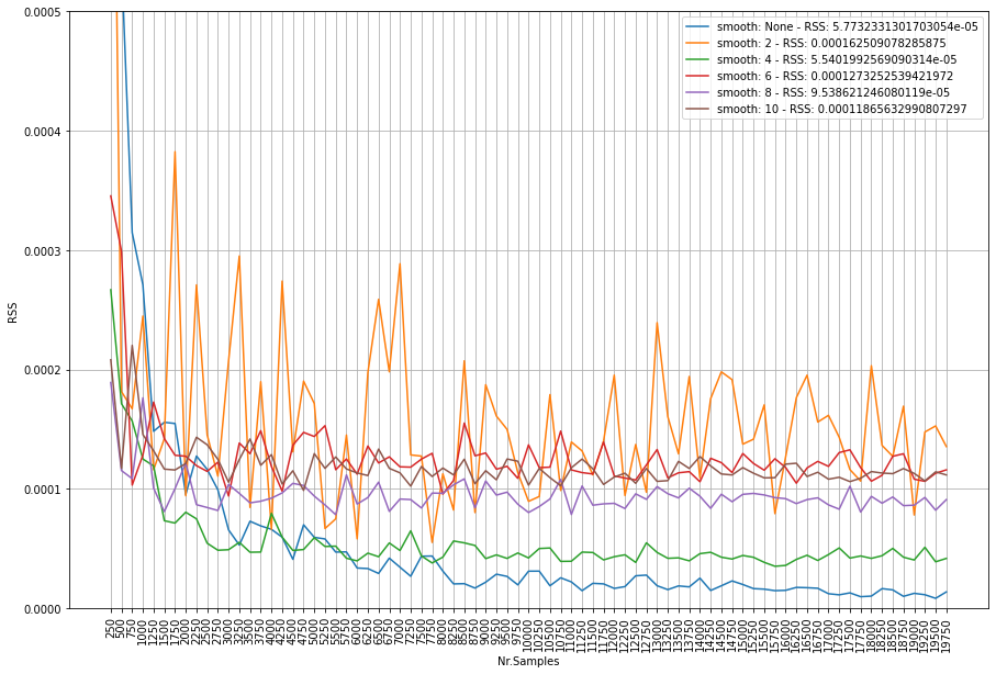
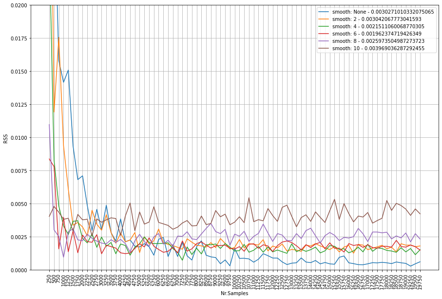
Lets analyze the RSS score acorss the varying sample sizes and smooting windows. The figure below depicts number of samples on the x-axis, and the RSS score on the y-axis. The lower the RSS score (towards zero) the better the fit. What we clearly see is that not smooting shows the best fit by an increasing number of samples (blue line). As an example, from 7000 samples, the smooting window does not improve the fitting at all anymore. The conlusion is that smooting seems only be effective for samples sizes lower then approximately 5000 samples. Note that this number may be different across data sets.
Integer fitting
It is recommend to fit integers using the method=discrete.
Here, I will demonstrate the effect of fitting a uniform distribution on integer values. lets generate random integer values from a uniform distribution, and examine the RSS scores. We will iterate over sample sizes and smoothing windows to analyze the performance.
import matplotlib.pyplot as plt
from tqdm import tqdm
import pandas as pd
import numpy as np
from distfit import distfit

# Sample sizes
samples = np.arange(250, 20000, 250)
# Smooting windows
smooth_window=[None, 2, 4, 6, 8, 10]

# Figure
plt.figure(figsize=(15,10))

# Iterate over smooting window
for smooth in tqdm(smooth_window):
# Fit only for the uniform distribution
    dfit = distfit(distr='uniform', smooth=smooth, stats='RSS', verbose=0)
    # Estimate paramters for the number of samples
    out = []

    # Iterate over sample sizes
    for s in samples:
        X = np.random.randint(0, 100, s)
        dfit.fit_transform(X)
        out.append([dfit.model['score'], dfit.model['name'], s])

    df = pd.DataFrame(out, columns=[dfit.stats,'name','samples'])
    ax=df[dfit.stats].plot(grid=True, label='smooth: '+str(smooth) + ' - RSS: ' + str(df[dfit.stats].mean()))

ax.set_xlabel('Nr.Samples')
ax.set_ylabel('RSS')
ax.set_xticks(np.arange(0,len(samples)))
ax.set_xticklabels(samples.astype(str))
ax.set_ylim([0, 0.001])
ax.legend()
The code above results in the underneath figure, where we have varying sample sizes on the x-axis, and the RSS score on the y-axis. The lower the RSS score (towards zero) the better the fit. What we clearly see is that orange is jumping up-and-down. This is smooting window=2. Tip: do not use this. Interesting to see is that not smooting shows the best fit by an increasing number of samples. Smooting does not improve the fitting anymore in case of more then 7000 samples. Note that this number may be different across data sets.
From these results we can conclude that smooting seems only usefull for small(er) samples sizes.