Quick start to find best fitting distribution
Specify distfit parameters. In this example nothing is specied and that means that all parameters are set to default.
Generate random data
from distfit import distfit
import numpy as np

# Example data
X = np.random.normal(10, 3, 2000)
y = [3,4,5,6,10,11,12,18,20]
Fit distributions
A series of distributions are fitted on the emperical data and for each a RSS is determined. The distribution with the best fit (lowest RSS) is the best fitting distribution.
# From the distfit library import the class distfit
from distfit import distfit

# Initialize
dfit = distfit(todf=True)

# Search for best theoretical fit on your empirical data
results = dfit.fit_transform(X)

# [distfit] >fit..
# [distfit] >transform..
# [distfit] >[norm      ] [0.00 sec] [RSS: 0.0036058] [loc=10.035 scale=2.947]
# [distfit] >[expon     ] [0.00 sec] [RSS: 0.1821936] [loc=-0.496 scale=10.531]
# [distfit] >[pareto    ] [0.12 sec] [RSS: 0.1821326] [loc=-699709.530 scale=699709.035]
# [distfit] >[dweibull  ] [0.02 sec] [RSS: 0.0059431] [loc=10.001 scale=2.541]
# [distfit] >[t         ] [0.09 sec] [RSS: 0.0036059] [loc=10.035 scale=2.947]
# [distfit] >[genextreme] [0.27 sec] [RSS: 0.7053157] [loc=17.658 scale=2.731]
# [distfit] >[gamma     ] [0.07 sec] [RSS: 0.0036036] [loc=-326.130 scale=0.026]
# [distfit] >[lognorm   ] [0.15 sec] [RSS: 0.0036144] [loc=-187.018 scale=197.039]
# [distfit] >[beta      ] [0.05 sec] [RSS: 0.0036176] [loc=-16.974 scale=51.538]
# [distfit] >[uniform   ] [0.00 sec] [RSS: 0.1162497] [loc=-0.496 scale=19.280]
# [distfit] >[loggamma  ] [0.07 sec] [RSS: 0.0036382] [loc=-493.477 scale=77.133]
# [distfit] >Compute confidence interval [parametric]
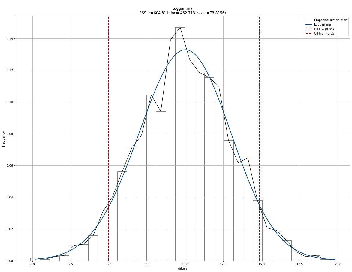
Plot distribution fit
# Plot
dfit.plot()
|
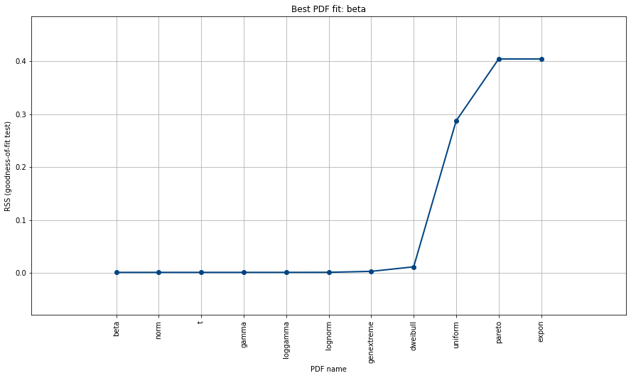
Plot RSS
Note that the best fit should be normal, as this was also the input data. However, many other distributions can be very similar with specific loc/scale parameters. It is however not unusual to see gamma and beta distribution as these are the “barba-pappas” among the distributions. Lets print the summary of detected distributions with the Residual Sum of Squares.
# Make plot
dfit.plot_summary()
|
Fit for one specific distribution
Suppose you want to test for one specific distribution, such as the normal distribution. This can be done as following:
# Create random data
X = np.random.normal(10, 3, 2000)
y = [3,4,5,6,10,11,12,18,20]

# Initialize
dfit = distfit(distr='norm')
# Fit on data
results = dfit.fit_transform(X)

# [distfit] >fit..
# [distfit] >transform..
# [distfit] >[norm] [RSS: 0.0151267] [loc=0.103 scale=2.028]

dfit.plot()
Fit for multiple distributions
Suppose you want to test multiple distributions:
# Create random data
X = np.random.normal(10, 3, 2000)
y = [3,4,5,6,10,11,12,18,20]

# Initialize
dfit = distfit(distr=['norm', 't', 'uniform'])
# Fit on data
results = dfit.fit_transform(X)

# [distfit] >fit..
# [distfit] >transform..
# [distfit] >[norm   ] [0.00 sec] [RSS: 0.0012337] [loc=0.005 scale=1.982]
# [distfit] >[t      ] [0.12 sec] [RSS: 0.0012336] [loc=0.005 scale=1.982]
# [distfit] >[uniform] [0.00 sec] [RSS: 0.2505846] [loc=-6.583 scale=15.076]
# [distfit] >Compute confidence interval [parametric]

dfit.plot()
Make predictions (continuous)
The predict function will compute the probability of samples in the fitted PDF.
Note that, due to multiple testing approaches, it can occur that samples can be located
outside the confidence interval but not marked as significant. See section Algorithm -> Multiple testing for more information.
Generate random data (continuous)
# Example data
X = np.random.normal(10, 3, 2000)
y = [3,4,5,6,10,11,12,18,20]
Fit all distribution
A series of distributions are fitted on the emperical data and for each a RSS is determined. The distribution with the best fit (lowest RSS) is the best fitting distribution.
# From the distfit library import the class distfit
from distfit import distfit

# Initialize
dfit = distfit(todf=True)

# Search for best theoretical fit on your empirical data
dfit.fit_transform(X)

# Make prediction on new datapoints based on the fit
results = dfit.predict(y)
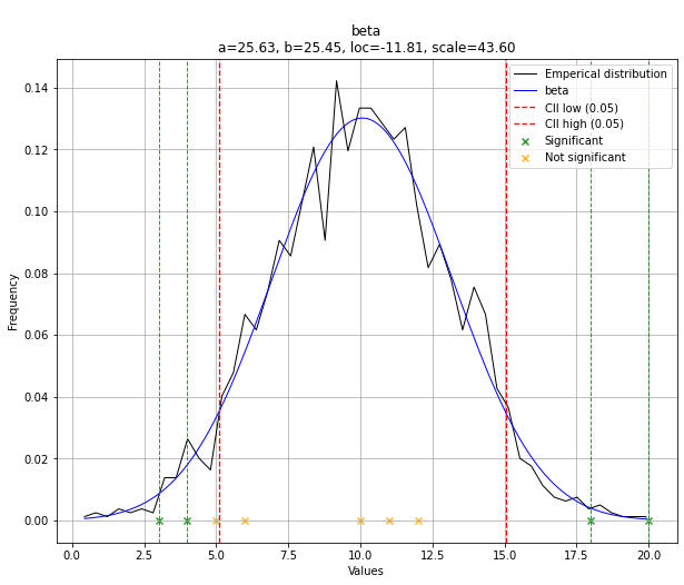
Plot predictions
The best fitted distribution is plotted over the emperical data with it confidence intervals.
# The plot function will now also include the predictions of y
dfit.plot()
Examine results
results is a dictionary containing y, y_proba, y_pred and P for which the output values has the same order as input value y.
The “P” stands for the RAW P-values and “y_proba” are the corrected P-values after multiple test correction (default: fdr_bh).
In case you want to use the “P” values, set “multtest” to None during initialization.
Note that dataframe df is included when using the todf=True parameter.
# Print probabilities
print(results['y_proba'])
# > [0.02702734, 0.04908335, 0.08492715, 0.13745288, 0.49567466, 0.41288701, 0.3248188 , 0.02260135, 0.00636084]

# Print the labels with respect to the confidence intervals
print(results['y_pred'])
# > ['down' 'down' 'down' 'none' 'none' 'none' 'none' 'up' 'up']

# Print the dataframe containing the total information
print(results['df'])
y |
y_proba |
y_pred |
P |
|
|---|---|---|---|---|
0 |
3 |
0.0270273 |
down |
0.00900911 |
1 |
4 |
0.0490833 |
down |
0.0218148 |
2 |
5 |
0.0849271 |
down |
0.0471817 |
3 |
6 |
0.137453 |
none |
0.0916353 |
4 |
10 |
0.495675 |
none |
0.495675 |
5 |
11 |
0.412887 |
none |
0.367011 |
6 |
12 |
0.324819 |
none |
0.252637 |
7 |
18 |
0.0226014 |
up |
0.00502252 |
8 |
20 |
0.00636084 |
up |
0.00070676 |
|
Output
In the previous example, we showed that the output can be captured results and out but the results are also stored in the object itself.
In our examples it is the dist object.
The same variable names are used; y, y_proba, y_pred and P.
Note that dataframe df is included when using the todf=True paramter.
# All scores of the tested distributions
print(dfit.summary)

# Distribution parameters for best fit
dfit.model

# Show the predictions for y
print(dfit.results['y_pred'])
# ['down' 'down' 'none' 'none' 'none' 'none' 'up' 'up' 'up']

# Show the probabilities for y that belong with the predictions
print(dfit.results['y_proba'])
# [2.75338375e-05 2.74664877e-03 4.74739680e-01 3.28636879e-01 1.99195071e-01 1.06316132e-01 5.05914722e-02 2.18922761e-02 8.89349927e-03]

# All predicted information is also stored in a structured dataframe (only when setting the todf=True)
# y: input values
# y_proba: corrected P-values after multiple test correction (default: fdr_bh).
# y_pred: True in case y_proba<=alpha
# P: raw P-values

print(dfit.results['df'])
y |
y_proba |
y_pred |
P |
|
|---|---|---|---|---|
0 |
3 |
0.0270273 |
down |
0.00900911 |
1 |
4 |
0.0490833 |
down |
0.0218148 |
2 |
5 |
0.0849271 |
down |
0.0471817 |
3 |
6 |
0.137453 |
none |
0.0916353 |
4 |
10 |
0.495675 |
none |
0.495675 |
5 |
11 |
0.412887 |
none |
0.367011 |
6 |
12 |
0.324819 |
none |
0.252637 |
7 |
18 |
0.0226014 |
up |
0.00502252 |
8 |
20 |
0.00636084 |
up |
0.00070676 |
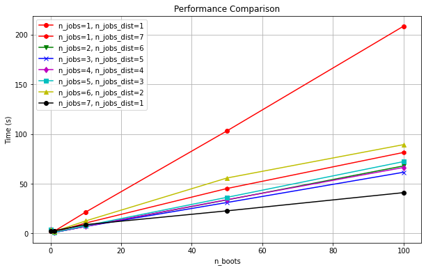
Parallel Computing
Distfit supports parallel computing where it performs parallelizing into two parts for maximum efficiency: over the fitting of distributions and separately over the bootstrap approach.
The chart below shows how effective parallelization is over these two parts. In general it can be seen that parallelizing is very effective! Time to compute is reduced from ~210sec to ~48sec.
The n_jobs_dist describes the general loop, while n_jobs pertains to the bootstrap part.
When the cores are somehow divided between the two tasks, there is no performance gain. In other words, when bootstrapping is enabled, it is best to allocate most of the cores to it.
Core allocation is automatically managed during initialization, so you only need to set n_jobs.
start_time = time.time()
# Initialization
dfit = distfit(distr='popular', n_boots=50, n_jobs=8, verbose='info')
# Fit
dfit.fit_transform(X)
# Compute time
elapsed_time = time.time() - start_time
print(elapsed_time)
|