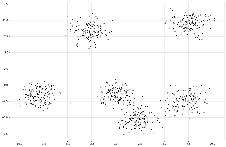
Generate data

Install requried libraries

pip install scatterd
pip install sklearn

Generate Data.

# Imports
from scatterd import scatterd
from clusteval import clusteval

# Init
cl = clusteval()

# Generate random data
X, y = cl.import_example(data='blobs')

# Scatter samples
scatterd(X[:,0], X[:,1], figsize=(15, 10));

Six circular clusters

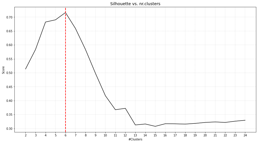
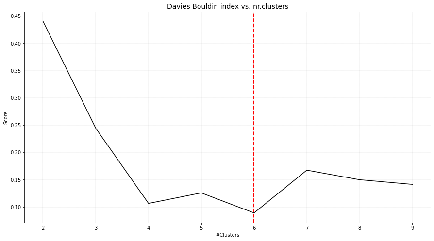
Plot

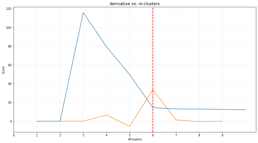
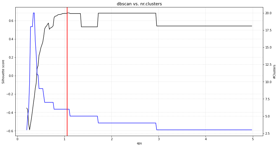
The plot functionality is to plot score of the cluster evaluation method versus the number of clusters. For demonstration, the clusters are evaluated using four cluster evaluation methods. It can be seen that all methods were able to detect the expected six clusters.

# Import
from clusteval import clusteval

# Silhouette cluster evaluation.
ce = clusteval(evaluate='silhouette')
# In case of using dbindex, it is best to clip the maximum number of clusters to avoid finding local minima.
ce = clusteval(evaluate='dbindex', max_clust=10)
# Derivative method.
ce = clusteval(evaluate='derivative')
# DBscan method.
ce = clusteval(cluster='dbscan')

# Fit
ce.fit(X)

# Plot
ce.plot()

Method vs. number of clusters

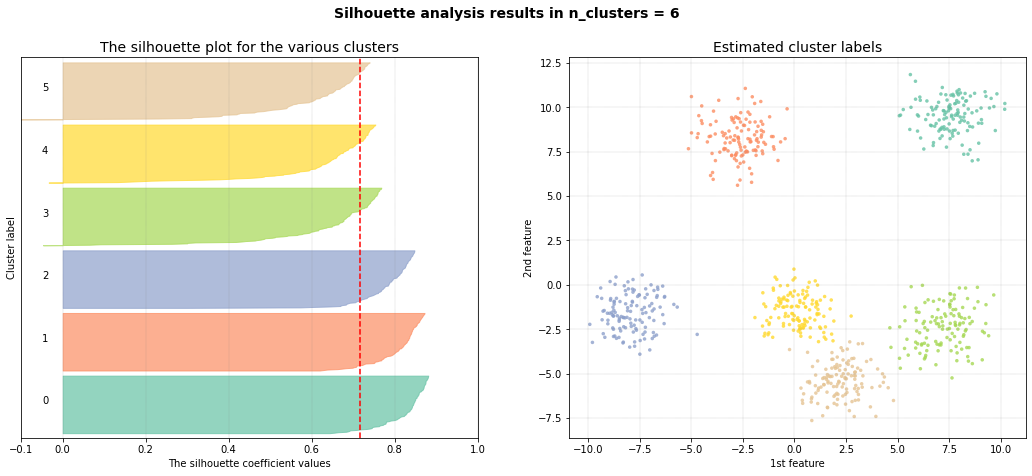
Silhouette plot

The aim of the scatterplot is to scatter the samples with the silhouette coefficient values. Note that for the scatterplot, only the first two features can be used.

# Plot Silhouette
ce.plot_silhouette()

Method vs. number of clusters for the silhouette method.

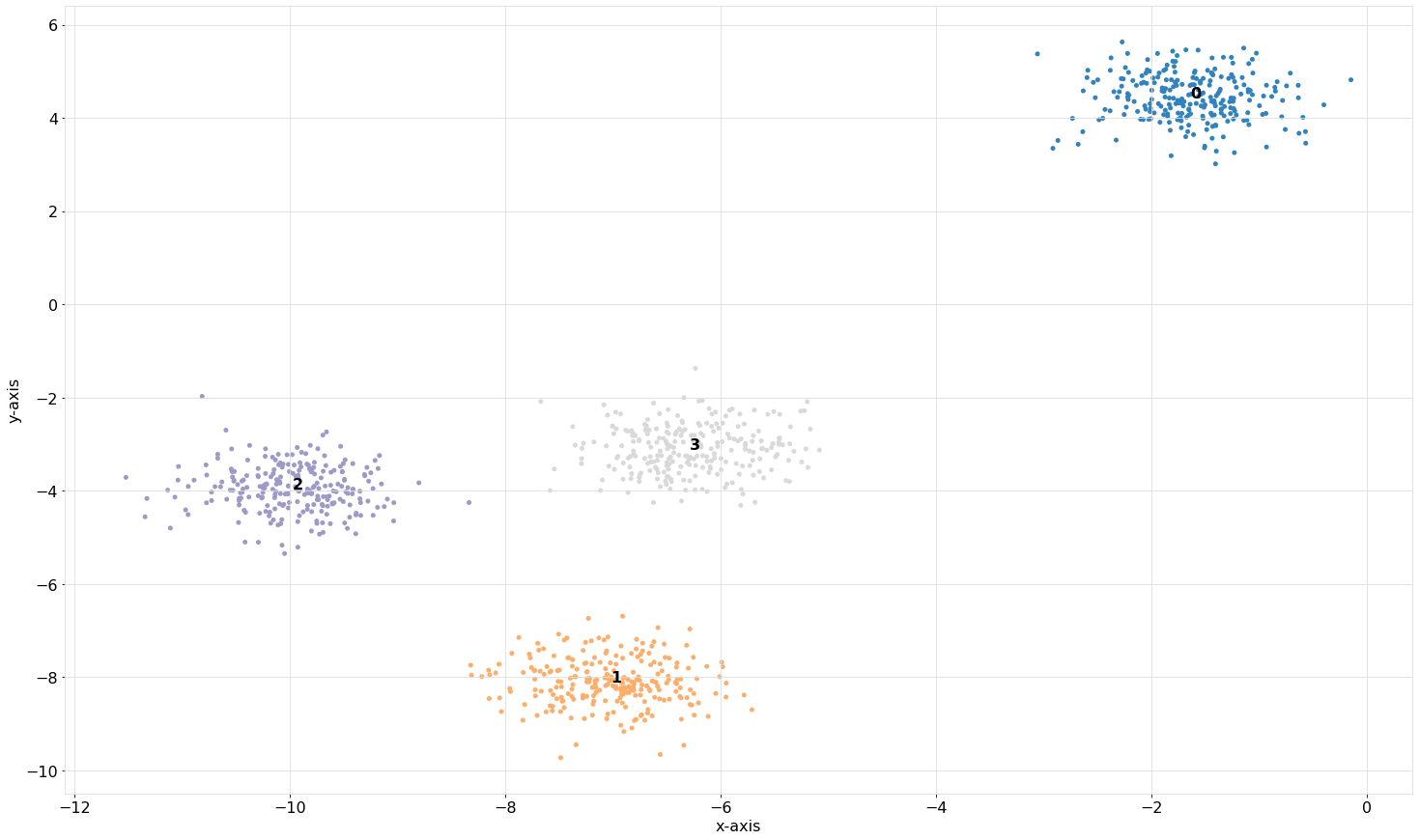
Scatter plot

The aim of the scatterplot is to scatter the samples with the silhouette coefficient values. Note that for the scatterplot, only the first two features can be used.

# Scatterplot
ce.scatter()

Scatterplot

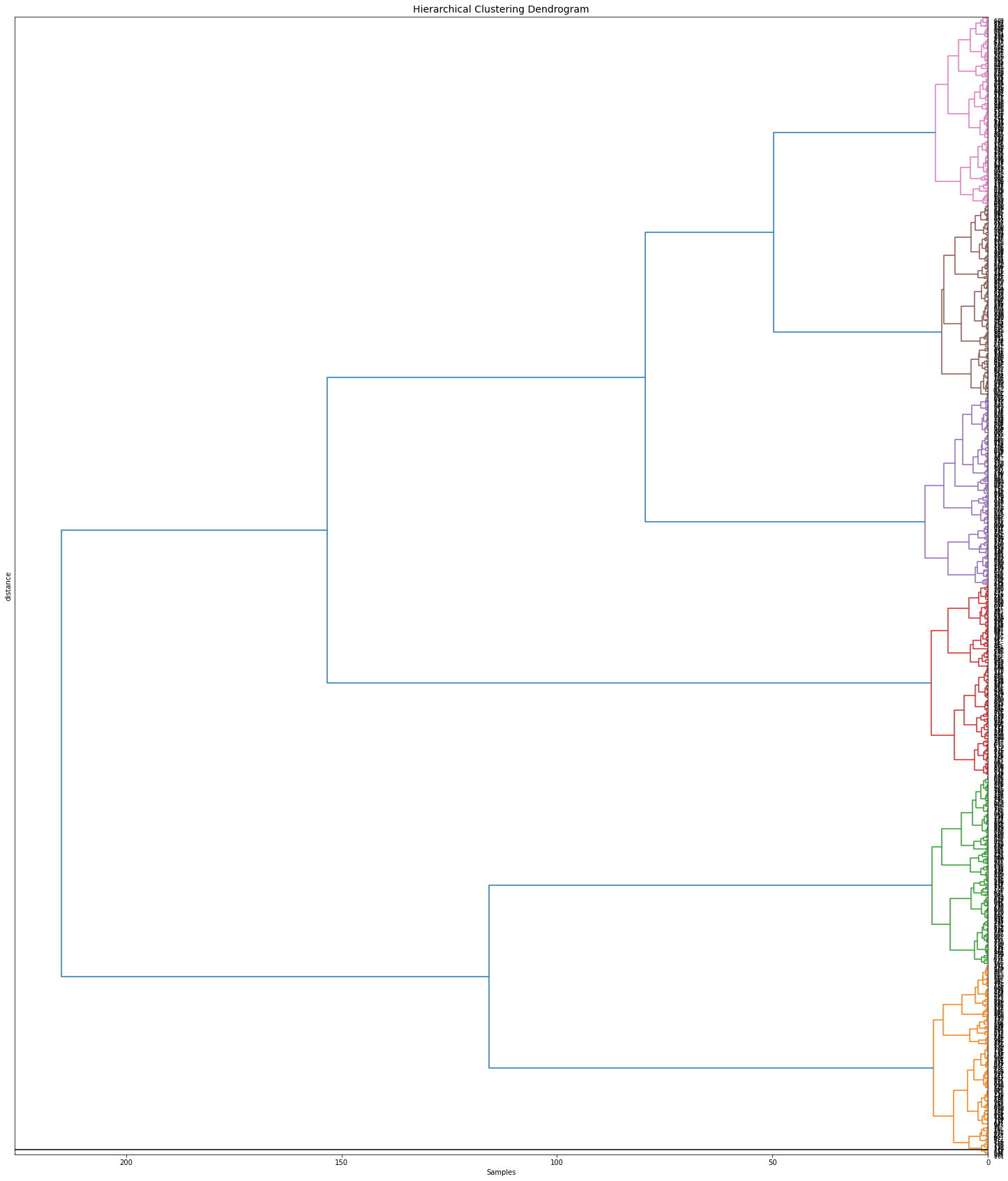
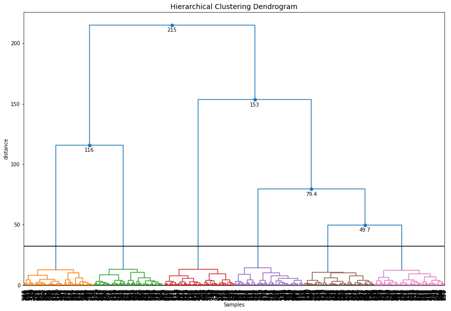
Dendrogram

Hierarchical tree plot

To furter investigate the clustering results, a dendrogram can be created.

ce.dendrogram()

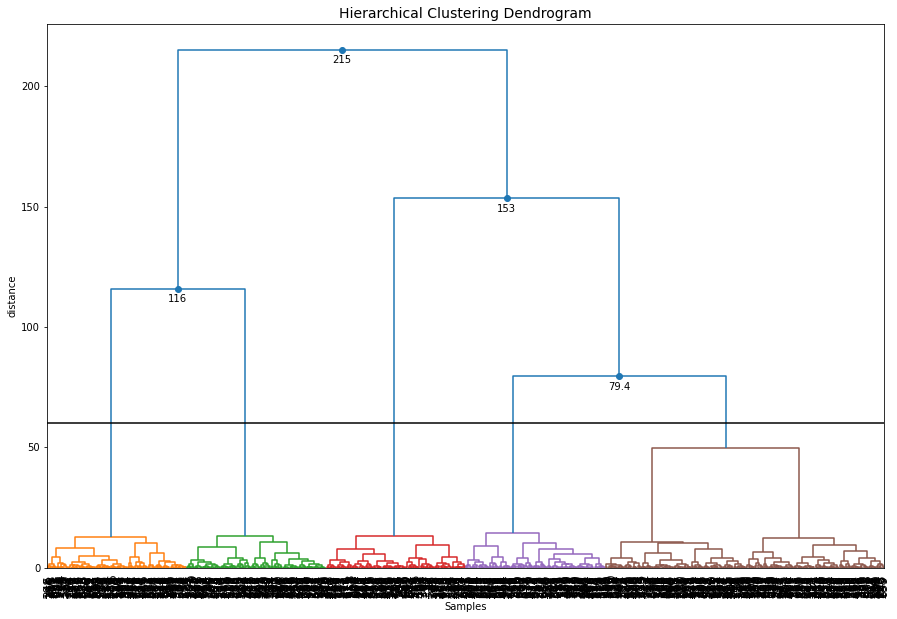
Change the cut-off threshold

The dendrogram function can now also be used to create differents cuts in the hierarchical clustering and retrieve the associated cluster labels. Let’s cut the tree at level 60

# Plot the dendrogram and make the cut at distance height 60
y = ce.dendrogram(max_d=60)

# Cluster labels for this particular cut
print(y['labx'])

Orientation

Change various parameters, such as orientation, leaf rotation, and the font size.

# Plot the dendrogram
ce.dendrogram(orientation='left', leaf_rotation=180, leaf_font_size=8, figsize=(25,30))

---

---