How to choose the cluster evaluation method?
With unsupervised clustering we aim to determine “natural” or “data-driven” groups in the data without using apriori knowledge about labels or categories. The challenge of using different unsupervised clustering methods is that it will result in different partitioning of the samples and thus different groupings since each method implicitly impose a structure on the data.
Note
There is no golden rule to define the optimal number of clusters. It requires investigation, and backtesting.
The implemented cluster evaluation methods works pretty well in certain scenarios but it requires to understand the mathematical properties of the methods so that it matches with the statistical properties of the data.
Investigate the underlying distribution of the data.
How should clusters “look” like? What is your aim?
Decide which distance metric, and linkage type is most appropriate for point 2.
Use the cluster evaluation method that fits best to the above mentioned points.
As an example: DBScan in combination with the Silhouette evaluation can detect clusters with different densities and shapes while k-means assumes that clusters are convex shaped. Or in other words, when using kmeans, you will always find convex shaped clusters!
Distance Metric
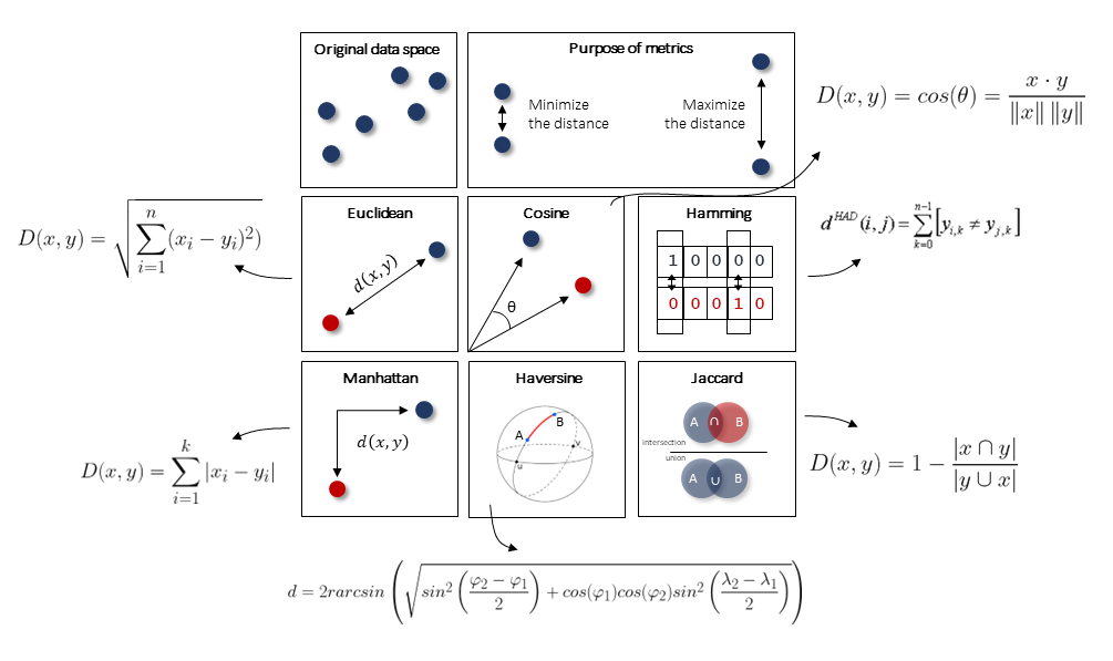
What is a “good” clustering? Intuitively, we may describe it as a group of samples that are cluttered together. However, it is better to describe clusters with the distances between the samples. The most well-known distance metric is the Euclidean distance. Although it is set as the default metric in many methods, it is not always the best choice. As an example, in case your dataset is boolean, then it is more wise to use a distance metric such as the hamming distance. Or in other words, use the metric that fits best by the statistical properties of your data.
|
Linkage types
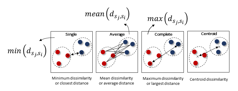
The process of hierarchical clustering involves an approach of grouping samples into a larger cluster. In this process, the distances between two sub-clusters need to be computed for which the different types of linkages describe how the clusters are connected. The most commonly used linkage type is complete linkage. Due to the nature of connecting groups, it can handle noisy data. However, if you aim to determine outliers or snake-like clusters, the single linkage is what you need.
|
Choose the metric and linkage type carefully because it directly affects the final clustering results. With this in mind, we can start preprocessing the images.
Note
Single linkage between two clusters is the proximity between their two closest samples. It produces a long chain and is therefore ideal to cluster spherical data but also for outlier detection.
Note
Complete linkage between two clusters is the proximity between their two most distant samples. Intuitively, the two most distant samples cannot be much more dissimilar than other quite dissimilar pairs. It forces clusters to be spherical and have often “compact” contours by their borders, but they are not necessarily compact inside.
Note
Average linkage between two clusters is the arithmetic mean of all the proximities between the objects of one, on one side, and the objects of the other, on the other side.
Note
Centroid linkage is the proximity between the geometric centroids of the clusters.
Derivative method
The “derivative” method is built on fcluster() from scipy. In clusteval, it compares each cluster merge’s height to the average and normalizes it by the standard deviation formed over the depth previous levels. Finally, the “derivative” method returns the cluster labels for the optimal cut-off based on the choosen hierarchical clustering method.
Let’s demonstrate this using the previously randomly generated samples.
# Libraries
from sklearn.datasets import make_blobs
from clusteval import clusteval

# Generate random data
X, _ = make_blobs(n_samples=500, centers=10, n_features=4, cluster_std=0.5)

# Intialize model
ce = clusteval(cluster='agglomerative', evaluate='derivative')

# Cluster evaluation
results = ce.fit(X)

# The clustering label can be found in:
print(results['labx'])

# Make plots
ce.plot()
ce.scatter(X)
ce.plot_silhouette(X)
Silhouette score
The silhouette method is a measure of how similar a sample is to its own cluster (cohesion) compared to other clusters (separation). The scores ranges between [−1, 1], where a high value indicates that the object is well matched to its own cluster and poorly matched to neighboring clusters. It is a sample-wise approach, which means that for each sample, a silhouette score is computed and if most samples have a high value, then the clustering configuration is appropriate. If many points have a low or negative value, then the clustering configuration may have too many or too few clusters.
In contrast to the DBindex, the Silhouette score is a sample-wise measure, i.e., measures the average similarity of the samples within a cluster and their distance to the other objects in the other clusters. The silhouette method is independent of the distance metrics which makes it an attractive and versatile method to use.
Note
Higher scores are better.
Tip
Independent of the distance metrics.
# Libraries
from sklearn.datasets import make_blobs
from clusteval import clusteval

# Generate random data
X, _ = make_blobs(n_samples=500, centers=10, n_features=4, cluster_std=0.5)

# Intialize model
ce = clusteval(cluster='agglomerative', evaluate='silhouette')

# Cluster evaluation
results = ce.fit(X)

# The clustering label can be found in:
print(results['labx'])

# Make plots
ce.plot()
ce.scatter(X)
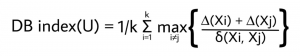
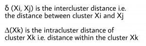
DBindex score
Davies–Bouldin index can intuitively be described as a measure of the ratio between within-cluster distances, and between cluster distances. The score is bounded between [0, 1]. The lower the value, the tighter the clusters and the seperation between clusters.
Note
Lower scores are better. However, it overshoots frequently. Use the “min_d” and “max_d” parameter to tune for the number of clusters.
Warning
Since it measures the distance between clusters centroids it is restricted to using the Euclidean distances.
|
|
# Libraries
from sklearn.datasets import make_blobs
from clusteval import clusteval

# Generate random data
X, _ = make_blobs(n_samples=500, centers=10, n_features=4, cluster_std=0.5)

# Intialize model
ce = clusteval(cluster='agglomerative', evaluate='dbindex')

# Cluster evaluation
results = ce.fit(X)

# The clustering label can be found in:
print(results['labx'])

# Make plots
ce.plot()
ce.scatter(X)
ce.dendrogram()
DBscan
Density-Based Spatial Clustering of Applications with Noise is an clustering approach that finds core samples of high density and expands clusters from them. This works especially good when having samples which contains clusters of similar density.
# Libraries
from sklearn.datasets import make_blobs
from clusteval import clusteval

# Generate random data
X, _ = make_blobs(n_samples=500, centers=10, n_features=4, cluster_std=0.5)

# Intialize model
ce = clusteval(cluster='dbscan')

# Parameters can be changed for dbscan:
# ce = clusteval(cluster='dbscan', params_dbscan={'epsres' :100, 'norm':True})

# Cluster evaluation
results = ce.fit(X)

# The clustering label can be found in:
print(results['labx'])

# Make plots
ce.plot()
ce.scatter(X)
HDBscan
Hierarchical Density-Based Spatial Clustering of Applications with Noise is an extension of the DBscan method which hierarchically finds core samples of high density and expands clusters from them.
Let’s evaluate the results using hdbscan.
pip install hdbscan
# Libraries
from sklearn.datasets import make_blobs
from clusteval import clusteval

# Generate random data
X, _ = make_blobs(n_samples=500, centers=10, n_features=4, cluster_std=0.5)

# Determine the optimal number of clusters
ce = clusteval(cluster='hdbscan')

# Make plots
ce.plot()
ce.scatter(X)