This section describes how to predict new unseen data points with a readily fitted model.
The find function clustimage.clustimage.Clustimage.find() allows to find images that are similar for what is readily being seen by the model. Finding images can be performed in two manners as described below. In both cases, the adjacency matrix is first computed using the distance metric (default Euclidean).
k-nearest neighbour
The k-nearest neighbour approach searches the k nearest neighbours to that of the input image using the (default) Euclidean distance metric. This approach dus not return a P-value the distances to the closest neighbors. If case both k and alpha are specified, the union of detected samples is taken.
Example to find similar samples for an unseen dataset using k-nearest neighbour approach.
from clustimage import Clustimage
import numpy as np

# Init with default settings
cl = Clustimage(method='pca')
# load example with digits
X, y = cl.import_example(data='mnist')

# Make 1st subset
idx = np.unique(np.random.randint(0,X.shape[0], 25))
X1 = X[idx, :]
X = X[np.setdiff1d(range(0, X.shape[0]), idx), :]

# Cluster dataset X
results = cl.fit_transform(X)
# Results are also stored in object results
cl.results.keys()
# Scatter results
cl.scatter(zoom=3, dotsize=50, figsize=(25, 15), legend=False, text=False)

# Find images for 1st subset of images
X1_results = cl.find(X1, k=5, alpha=None)
# Make scatter
cl.scatter(zoom=5, dotsize=100, text=False, figsize=(35, 20))

# Print first key
keys = list(X1_results.keys())[1:]
print(X1_results.get(keys[0]).columns)
# ['y_idx', 'distance', 'y_proba', 'labels', 'y_filenames', 'y_pathnames', 'x_pathnames']

print(X1_results.get(keys[0])[['labels', 'distance','y_proba']])
#    labels    distance  y_proba
# 0       9  189.436546      NaN
# 1       9  305.387050      NaN
# 2       9  338.403554      NaN
# 3       9  342.050496      NaN
# 4       9  351.139465      NaN

# Get most often seen class label for key
for key in keys:
    uiy, ycounts = np.unique(X1_results.get(key)['labels'], return_counts=True)
    y_predict = uiy[np.argmax(ycounts)]
    print('class:[%s] - %s' %(y_predict, key))

# class:[9] - b2ea44d9-de55-421b-8bd1-6d13509533f5.png
# class:[4] - 60dabaf0-7e1a-4c57-bb57-5d464fd2d8fb.png
# class:[6] - dbc30522-5c83-4563-9c9f-40a86f24a091.png
# class:[1] - deb11282-a992-4282-8212-ba62ef1e26fc.png
# class:[3] - 29104a7c-775b-462f-84ba-e824c7c4b9c7.png
# class:[9] - 45e6f5fd-4423-4743-850e-921914bfb9c9.png
# class:[9] - 300a866e-5440-444a-b284-d2bfb1b1178b.png
# class:[8] - 2dd0defc-d72a-4189-abae-bd33a94ee044.png
# class:[7] - a308d13e-fa3e-4428-8b5e-edb26554d723.png
# class:[2] - 6dc9c2b5-e1eb-4b6e-891a-db657c663013.png
# class:[9] - 30477a7a-e7a0-44f2-8bb2-222719ebe12b.png
# class:[5] - 50261737-f812-4665-b46f-cf8afb3cc88c.png
# class:[0] - c83ab55a-2983-44a6-9e2e-4964dc13c1b0.png
# class:[9] - 3eafd007-b6ed-4d17-a9db-3477854525df.png
# class:[8] - 411c207e-4804-4e30-a1c5-546876e36c51.png
# class:[4] - 661ac0f2-6f41-493a-bb3a-2c068c632d86.png
# class:[9] - 9fc65ef1-ff93-4ac6-9cdb-f4605ee9661a.png
# class:[7] - 6d9e017e-fc6a-424f-8f40-52995db771dc.png
# class:[4] - dfc5cf51-2157-437f-b1ce-920100b74119.png
# class:[4] - 507c365d-d35d-4623-985a-e9512c511d11.png
# class:[0] - 058f3759-2608-490e-ac79-e5fde8d10f7e.png
# class:[2] - a10dbae8-81f1-4613-8fd9-0bfa4815f1ad.png
# class:[2] - a889af11-961c-42f6-8b34-3d0f7050c34c.png
# class:[0] - 2e92d26c-3bf4-4c25-9d7e-4ceaa2e06d69.png
# class:[4] - b7706e78-c653-4e26-9d7a-bcb512751526.png
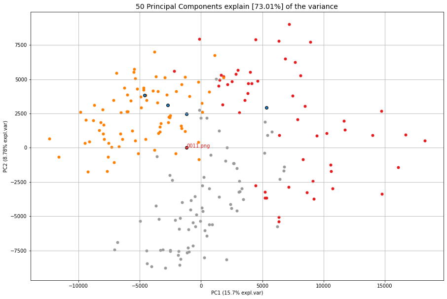
Probability density fitting
The probability density fitting method fits a model on the input features to determine the loc/scale/arg parameters across various theoretical distribution. In case of PCA, these are the principal components. The tested disributions are [‘norm’, ‘expon’, ‘uniform’, ‘gamma’, ‘t’]. The fitted distribution is the similarity-distribution of samples.
For each new (unseen) input image, the probability of similarity is computed across the images, and images with P <= *alpha*(lower bound) are returned. Note that the metric can be changed in this function but this may lead to confusions as the results will not intuitively match with the scatter plots as these are determined using metric in the fit_transform() function.
Example to find similar samples for an unseen dataset using probability density fitting.
from clustimage import Clustimage
import numpy as np

# Init with default settings
cl = Clustimage(method='pca')
# load example with digits
X, y = cl.import_example(data='mnist')

# Make 1st subset
idx = np.unique(np.random.randint(0,X.shape[0], 25))
X1 = X[idx, :]
X = X[np.setdiff1d(range(0, X.shape[0]), idx), :]

# Cluster dataset X
results = cl.fit_transform(X)
# Results are also stored in object results
cl.results.keys()
# Scatter results
cl.scatter(zoom=3, dotsize=50, figsize=(25, 15), legend=False, text=False)

# Find images for 1st subset of images
X1_results = cl.find(X1, alpha=0.05)
# Make scatter
cl.scatter(zoom=5, dotsize=100, text=False, figsize=(35, 20))

# Print first key
keys = list(X1_results.keys())[1:]
print(X1_results.get(keys[0]).columns)
# ['y_idx', 'distance', 'y_proba', 'labels', 'y_filenames', 'y_pathnames', 'x_pathnames']
print(X1_results.get(keys[0])[['labels', 'distance','y_proba']])

#     labels    distance   y_proba
# 0        8  189.373756  0.000035
# 1        8  305.290164  0.000822
# 2        8  338.588849  0.001812
# 3        8  341.933366  0.001956
# 4        8  351.231864  0.002412
# ..     ...         ...       ...
# 57       8  506.617886  0.044141
# 58       8  507.522983  0.044750
# 59       8  508.852247  0.045657
# 60       8  509.517201  0.046116
# 61       8  511.862011  0.047765

# Get most often seen class label for key
for key in keys:
    uiy, ycounts = np.unique(X1_results.get(key)['labels'], return_counts=True)
    y_predict = uiy[np.argmax(ycounts)]
    print('class:[%s] - %s' %(y_predict, key))

# class:[9] - b2ea44d9-de55-421b-8bd1-6d13509533f5.png
# class:[4] - 60dabaf0-7e1a-4c57-bb57-5d464fd2d8fb.png
# class:[6] - dbc30522-5c83-4563-9c9f-40a86f24a091.png
# class:[1] - deb11282-a992-4282-8212-ba62ef1e26fc.png
# class:[3] - 29104a7c-775b-462f-84ba-e824c7c4b9c7.png
# class:[9] - 45e6f5fd-4423-4743-850e-921914bfb9c9.png
# class:[9] - 300a866e-5440-444a-b284-d2bfb1b1178b.png
# class:[8] - 2dd0defc-d72a-4189-abae-bd33a94ee044.png
# class:[7] - a308d13e-fa3e-4428-8b5e-edb26554d723.png
# class:[2] - 6dc9c2b5-e1eb-4b6e-891a-db657c663013.png
# class:[9] - 30477a7a-e7a0-44f2-8bb2-222719ebe12b.png
# class:[5] - 50261737-f812-4665-b46f-cf8afb3cc88c.png
# class:[0] - c83ab55a-2983-44a6-9e2e-4964dc13c1b0.png
# class:[9] - 3eafd007-b6ed-4d17-a9db-3477854525df.png
# class:[8] - 411c207e-4804-4e30-a1c5-546876e36c51.png
# class:[4] - 661ac0f2-6f41-493a-bb3a-2c068c632d86.png
# class:[9] - 9fc65ef1-ff93-4ac6-9cdb-f4605ee9661a.png
# class:[7] - 6d9e017e-fc6a-424f-8f40-52995db771dc.png
# class:[4] - dfc5cf51-2157-437f-b1ce-920100b74119.png
# class:[4] - 507c365d-d35d-4623-985a-e9512c511d11.png
# class:[0] - 058f3759-2608-490e-ac79-e5fde8d10f7e.png
# class:[2] - a10dbae8-81f1-4613-8fd9-0bfa4815f1ad.png
# class:[2] - a889af11-961c-42f6-8b34-3d0f7050c34c.png
# class:[0] - 2e92d26c-3bf4-4c25-9d7e-4ceaa2e06d69.png
# class:[4] - b7706e78-c653-4e26-9d7a-bcb512751526.png
More examples
from clustimage import Clustimage
import matplotlib.pyplot as plt
import pandas as pd
# Init with default settings
cl = Clustimage(method='pca')
# load example with digits
X, y = cl.import_example(data='mnist')
# Cluster digits
results = cl.fit_transform(X)
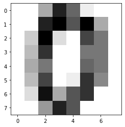
# Lets search for the following image:
plt.figure(); plt.imshow(X[0,:].reshape(cl.params['dim']), cmap='binary')
# Find images
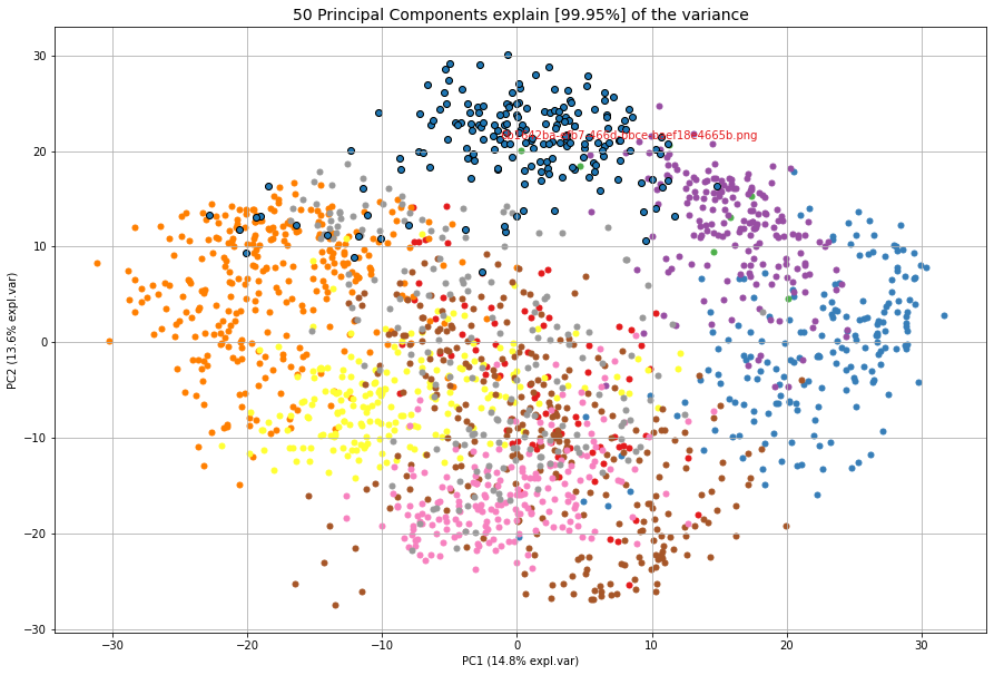
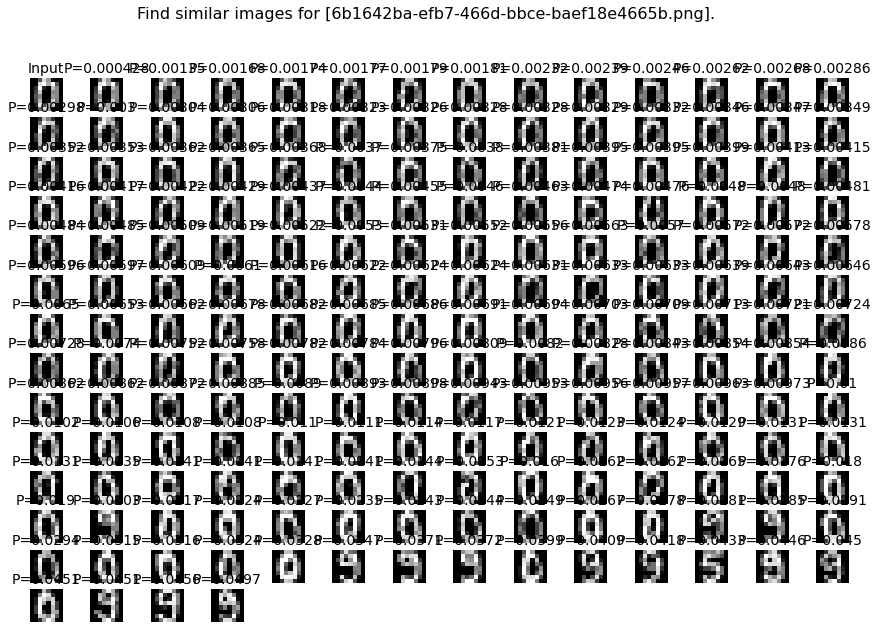
results_find = cl.find(X[0:3,:], k=None, alpha=0.05)
# Show whatever is found. This looks pretty good.
cl.plot_find()
cl.scatter(zoom=3)
# Extract the first input image name
filename = [*results_find.keys()][1]
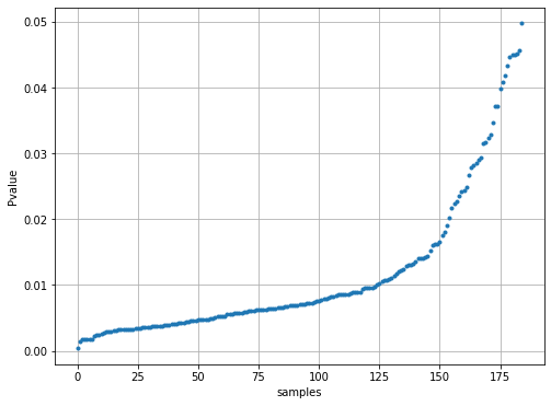
# Plot the probabilities
plt.figure(figsize=(8,6))
plt.plot(results_find[filename]['y_proba'],'.')
plt.grid(True)
plt.xlabel('samples')
plt.ylabel('Pvalue')
# Extract the cluster labels for the input image
results_find[filename]['labels']
# The majority of labels is for class 0
print(pd.value_counts(results_find[filename]['labels']))
# 0 171
# 7 8
# Name: labels, dtype: int64
|
|
|
|
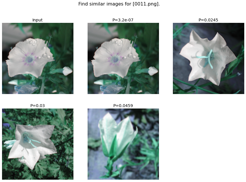
** Example to find similar images based on the pathname as input.**
from clustimage import Clustimage

# Init with default settings
cl = Clustimage(method='pca')

# load example with flowers
pathnames = cl.import_example(data='flowers')

# Cluster flowers
results = cl.fit_transform(pathnames[1:])

# Lets search for the following image:
img = cl.imread(pathnames[10], colorscale=1)
plt.figure(); plt.imshow(img.reshape((128,128,3)));plt.axis('off')

# Find images
results_find = cl.find(pathnames[10], k=None, alpha=0.05)

# Show whatever is found. This looks pretty good.
cl.plot_find()
cl.scatter()
|
|