PCA
Principal component analysis (PCA) is a feature extraction approach for which we can leverage on the first few principal components and ignoring the rest.
In clustimage the pca library utilized to extract the first 50 (default) components.
The use of PC’s for clustering is usefull in applications with among others faces, where so called eigenfaces are computed.
The eigenface is a low-dimensional representation of face images. It is shown that principal component analysis could be used on a collection of face images to form a set of basis features.
# Initialize with pca and 50 PCs
cl = Clustimage(method='pca', params_pca={'n_components':50})
# Take the number of components that covers 95% of the data
cl = Clustimage(method='pca', params_pca={'n_components':0.95})

# Load example data
X, y = cl.import_example(data='mnist')

# Check whether in is dir, list of files or array-like
X = cl.import_data(X)
# Extract features using method
Xfeat = cl.extract_feat(X)
# Alternatively, the features are also stored in the results dict
cl.results['feat']

# Alternatively, the features are also stored in the results dict using the run-at-once function.
results = cl.fit_transform(X)
# Extracted PC features
results['feat']
HOG
Histogram of Oriented Gradients (HOG), is a feature descriptor that is often used to extract features from image data. In general, it is a simplified representation of the image that contains only the most important information about the image. The HOG feature descriptor counts the occurrences of gradient orientation in localized portions of an image. It is widely used in computer vision tasks for object detection.
The HOG descriptor focuses on the structure or the shape of an object. Note that this is different then edge features that we can extract for images because in case of HOG features, both edge and direction are extracted.
The complete image is broken down into smaller regions (localized portions) and for each region, the gradients and orientation are calculated.
Finally the HOG would generate a Histogram for each of these regions separately. The histograms are created using the gradients and orientations of the pixel values, hence the name Histogram of Oriented Gradients
Not all applications are usefull when using HOG features as it “only” provides the outline of the image. For example, if the use-case is to group faces or cars, HOG-features can do a great job but a deeper similarity of faces or types of cars may be difficult as the details will be losed.
The input parameters for the HOG function clustimage.clustimage.Clustimage.extract_hog()
image vector : Flattened 1D vector of the image
orientations : number of allowed orientations (default is 8)
pixels_per_cell : Number of pixels per cell aka the HOG-resolution (default: 16, 16)
cells_per_block : number of cells per block (default: 1, 1).
    # Initialize with HOG
    cl = Clustimage(method='hog', params_hog={'orientations':8, 'pixels_per_cell':(8,8), 'cells_per_block':(1,1)})

    # Load example data
    X, y = cl.import_example(data='mnist')

    # Check whether in is dir, list of files or array-like
    X = cl.import_data(X)

    # Extract features using method
    Xfeat = cl.extract_feat(X)

    # The features are also stored in the results dict
    cl.results['feat']

    # Take one image and show the hog features
Xhog = cl.results['feat'][55]
Ximg = cl.results['img'][55]

plt.figure()
fig,axs=plt.subplots(1,2, figsize=(15,10))
axs[0].imshow(Ximg.reshape(8, 8))
axs[0].axis('off')
axs[0].set_title('Preprocessed image', fontsize=12)
axs[1].imshow(Xhog.reshape(8, 8), cmap='gray')
axs[1].axis('off')
axs[1].set_title('HOG', fontsize=12)
Another approach to extract HOG features by directly using the extract_hog functionality:
import matplotlib.pyplot as plt
from clustimage import Clustimage

# Init
cl = Clustimage(method='hog')

# Load example data
pathnames = cl.import_example(data='flowers')

# Read image according the preprocessing steps
img = cl.imread(pathnames[10], dim=(128,128))

# Extract HOG features
img_hog = cl.extract_hog(img, pixels_per_cell=(8,8), orientations=8, flatten=False)

plt.figure()
fig,axs=plt.subplots(1,2, figsize=(15,10))
axs[0].imshow(img.reshape(128,128,3))
axs[0].axis('off')
axs[0].set_title('Preprocessed image', fontsize=12)
axs[1].imshow(img_hog, cmap='gray')
axs[1].axis('off')
axs[1].set_title('HOG', fontsize=12)
|
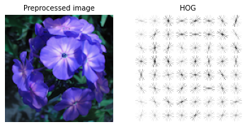
Here it can be clearly seen that the HOG image is a matrix of 8x8 vectors that is derived by because of the input image (128,128) devided by the pixels per cell (16,16). Thus 128/16=8 rows and columns in this case. If an increase of HOG features is desired, you can either increasing the image dimensions (eg 256,256) or decrease the pixels per cell (eg 8,8).
EXIF
EXIF (Exchangeable Image File Format) metadata is embedded in most image files and contains valuable information such as timestamps, GPS coordinates, and camera settings. This data can be utilized for clustering images, especially based on datetime and lat/lon data. Below, we explain how to achieve this, step by step.
There are two metric where EXIF metadata is used for clustering:
‘latlon’: Cluster files on lon/lat coordinates.
‘datetime’: Cluster files on date/time.
Each approach can be tuned by a few parameters that can be set using params_exif.
params_exif: dict, default: {'timeframe': 6, 'radius_meters': 1000, 'exif_location': False}
‘timeframe’: The timeframe in hours that is used to group the images.
‘radius_meters’: The radius that is used to cluster the images when using metric=’datetime’
‘exif_location’: This function makes requests to derive the location such as streetname etc. Note that the request rate per photo limited to 1 sec to prevent time-outs. It requires photos with lat/lon coordinates and is not used in the clustering. This information is only used in the plot.
Clustering by Datetime
Clustering files by datetime can help organize or analyze images captured within specific time intervals, such as during an event or over consecutive hours or days. For each file, the EXIF datetime creation date is extracted when possible. If the datetime information could not be found in the EXIF data, the file timestamp will be used instead. However, the latter can cause that the modified time is used instead of creation time depending on the operating system. The advantage of this approach is that it allows to cluster on more then only image files, all files are allowed such as .mp4, .mov or .txt etc files. This approach will therefore help you to easily organize your directory of images together with movies etc.
from clustimage import Clustimage

# Init
cl = Clustimage(method='exif',
                params_exif = {'timeframe': 6, 'min_samples': 2, 'exif_location': False},
                ext=["mp4", "mov", "jpg", "jpeg", "png", "tiff", "bmp", "gif", "webp", "psd", "raw", "cr2", "nef", "heic", "sr2", "tif"],
                verbose='info')

# Path to your images or photos
dir_path = r'c:/temp/'

# Run the model to find Clusters of photos within the same timeframe
# blacklist does block the images in the "undouble" directory
# recursive will search for images in also all subdirectories
results = cl.fit_transform(dir_path, metric='datetime', min_clust=3, black_list=['undouble'], recursive=True)

# Show the cluster labels.
# Note that cluster 0 is the "rest" group
print(cl.results['labels'])

# Make plot but exclude cluster 0 (rest group).
# Only create a plot when the cluster contains 4 or more images.
cl.plot(blacklist=[0], min_samples=4)

# plot on Map
# polygon: See the lines in which order the photos were created
# cluster_icons: automatically groups icons when zooming in/out. When enabled, the exact lat/lon is not used but an approximate.
# save_path: Store path. When not used, it will be stored in the temp directory
cl.plot_map(cluster_icons=False, open_in_browser=True, polygon=True, save_path=os.path.join(dir_path, 'map.html'))
Clustering by Latlon
Geographic data embedded in EXIF metadata allows images to be clustered by their GPS coordinates, enabling grouping by physical proximity (e.g., taken in the same city, park, or venue).
This approach extract GPS latitude and longitude Coordinates from EXIF Metadata and then clusters using DBSCAN (can not be changed).
from clustimage import Clustimage

# Init
cl = Clustimage(method='exif',
                params_exif = {radius_meters': 1000, 'min_samples': 2, 'exif_location': False},
                ext=["jpg", "jpeg", "png", "tiff", "bmp", "gif", "webp", "psd", "raw", "cr2", "nef", "heic", "sr2", "tif"],
                verbose='info')

# Path to your images or photos
dir_path = r'c:/temp/'

# Run the model to find Clusters of photos within the same lat/lon with a radius of 1000 meters
# blacklist does block the images in the "undouble" directory
# recursive will search for images in also all subdirectories
results = cl.fit_transform(dir_path, metric='latlon', min_clust=3, black_list=['undouble'], recursive=True)

# Show the cluster labels.
# Note that cluster 0 is the "rest" group
print(cl.results['labels'])

# Make plot but exclude cluster 0 (rest group).
# Only create a plot when the cluster contains 4 or more images.
cl.plot(blacklist=[0], min_samples=4)

# plot on Map
# polygon: Disable the lines in which order the photos were created because it will likely not make sense here.
# cluster_icons: automatically groups icons when zooming in/out. When enabled, the exact lat/lon is not used but an approximate.
# save_path: Store path. When not used, it will be stored in the temp directory
cl.plot_map(cluster_icons=True, open_in_browser=True, polygon=False, save_path=os.path.join(dir_path, 'map.html'))