Methods
The classeval library contains various measures to estimate the models performance.
The main function to evaluated models performance is the function classeval.classeval.eval().
This function automatically determines whether your trained model is based on a two-class or multi-class approach.
Two-class approach
Two-class models are trained on two classes; the class-of-interest versus the rest-class. Such approach is commonly used across image-recognition, network-analysis, sensor data or any other type of data.
The classeval.classeval.eval() function requires three input parameters. It is also possible to directly use the two-class function classeval.classeval.eval_twoclass(), the outputs are identical.
- Parameters required
y_true : The true class label
y_proba : Probability of the predicted class label
y_pred : Predicted class label
Multi-class approach
Multi-class models are trained on… Yes, multiple classes. These models are often used in textmining where the number of classes are high as these usually represent various textual catagories.
A disadvantage of multi-class models is a higher model complexity and many generic performance statistics can not be used.
The classeval.classeval.eval() function requires three input parameters. It is also possible to directly use the classeval.classeval.eval_multiclass(). Here, the outputs are also identifical.
- Parameters required
y_true : The true class label
y_proba : Probability of the predicted class label
y_score : Model decision function
Optimizing model performance
The classeval library can also help in tuning the models performance by examining the effect of the threshold.
After learning a model, and predicting new samples with it, each sample will get a probability belowing to the class.
In case of our two-class approach the simple rule account: P(class-of-interest) = 1-P(not class-of-interest)
Evaluation methods
Confusion-matrix
A confusion matrix is a table that is used to describe the performance of a classification model on a set of test data for which the true values are known.
The function is callable by func:classeval.confmatrix.eval and the plot can be created with func:classeval.confmatrix.plot
- Applicable
Two-class approach
multi-class approach
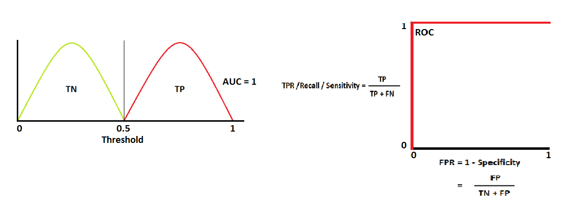
ROC/AUC
The Area Under The Curve (AUC) and Receiver Operating Characteristics curve (ROC) are one of the most important evaluation metrics for checking any classification model’s performance. The goal of the AUC-ROC is to determine the probability curve and degree or measure of separability by using various thresholds settings. It describes how much the model is capable of distinguishing between the classes. The higher the AUC, the better the model is at predicting whereas a AUC of 0.5 represents random results.
In case of a multi-class approach, the AUC is computed using the One-vs-Rest scheme (OvR) and One-vs-One scheme (OvO) schemes.
The multi-class One-vs-One scheme compares every unique pairwise combination of classes. Macro average, and a prevalence-weighted average.
This function is callable via: classeval.classeval.AUC_multiclass()
The function is callable by func:classeval.ROC.eval and the plot can be created with func:classeval.ROC.plot
- Applicable
Two-class approach
multi-class approach
A perfect score would result in an AUC score=1 and ROC curve like this:
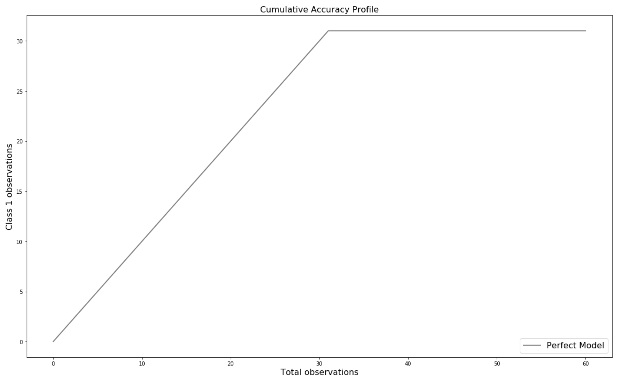
CAP analysis
The CAP Curve analyse how to effectively identify all data points of a given class using minimum number of tries. This function computes Cumulitive Accuracy Profile (CAP) to measure the performance of a classifier. It ranks the predicted class probabilities (high to low), together with the true values. With that, it computes the cumsum which is the final line. A perfect model is one which will detect all class 1.0 data points in the same number of tries as there are class 1.0 data points.
This function is callable with: classeval.classeval.CAP()
- Applicable
Two-class approach
- A perfect score would result in an CAP score=100 and CAP. Note that if the value is more than 90%, it’s a good practice to test for over fitting.
More than 90%: Too Good to be True
80% — 90%: Very Good Model
70% — 80%: Good Model
60% — 70%: Poor Model
Less than 60%: Rubbish Model
Average Precision (AP)
A better metric in an imbalanced situation is the AUC PR (Area Under the Curve Precision Recall), or also called AP (Average Precision). If the precision decreases when we increase the recall, it shows that we have to choose a prediction thresold adapted to our needs. If our goal is to have a high recall, we should set a low prediction thresold that will allow us to detect most of the observations of the positive class, but with a low precision. On the contrary, if we want to be really confident about our predictions but don’t mind about not finding all the positive observations, we should set a high thresold that will get us a high precision and a low recall. In order to know if our model performs better than another classifier, we can simply use the AP metric. To assess the quality of our model, we can compare it to a simple decision baseline.
Let’s take a random classifier as a baseline here that would predict half of the time 1 and half of the time 0 for the label. Such a classifier would have a precision of 4.3%, which corresponds to the proportion of positive observations. For every recall value the precision would stay the same, and this would lead us to an AP of 0.043. The AP of our model is approximately 0.35, which is more than 8 times higher than the AP of the random method. This means that our model has a good predictive power.
This function is callable with: classeval.classeval.AP()
- Applicable
Two-class approach
Imbalanced classes
F1-score
The F1 score (also F-score or F-measure) is a measure of a test’s accuracy. It considers both the precision p and the recall r of the test to compute the score: p is the number of correct positive results divided by the number of all positive results returned by the classifier, and r is the number of correct positive results divided by the number of all relevant samples (all samples that should have been identified as positive).

- Applicable
Two-class approach
Kappa
In essence, the kappa statistic is a measure of how closely the instances classified by the machine learning classifier matched the data labeled as ground truth, controlling for the accuracy of a random classifier as measured by the expected accuracy. In some other cases we might face a problem with imbalanced classes. E.g. we have two classes, say A and B, and A shows up on 5% of the time. Accuracy can be misleading, so we go for measures such as precision and recall. There are ways to combine the two, such as the F-measure, but the F-measure does not have a very good intuitive explanation, other than it being the harmonic mean of precision and recall. Cohen’s kappa statistic is a very good measure that can handle very well both multi-class and imbalanced class problems.
- Applicable
Two-class approach
Imbalanced classes
As an example, suppose we have the following results as depicted in the confusion matrix:
normal
defect
normal
22
9
defect
7
13
Ground truth: normal (29), defect (22)
Machine Learning Classifier: normal (31), defect (20)
Total: (51)
Observed Accuracy: ((22 + 13) / 51) = 0.69
Expected Accuracy: ((29 * 31 / 51) + (22 * 20 / 51)) / 51 = 0.51
Kappa: (0.69 - 0.51) / (1 - 0.51) = 0.37
Kappa values below 0 are possible, Cohen notes they are unlikely in practice.
MCC
MCC is extremely good metric for the **imbalanced* classification.*
- Score Ranges between [−1,1], where:
1 : Perfect prediction
0 : Random prediction
−1: Total disagreement between predicted scores and true labels values.
- Applicable
Two-class approach
Imbalanced classes
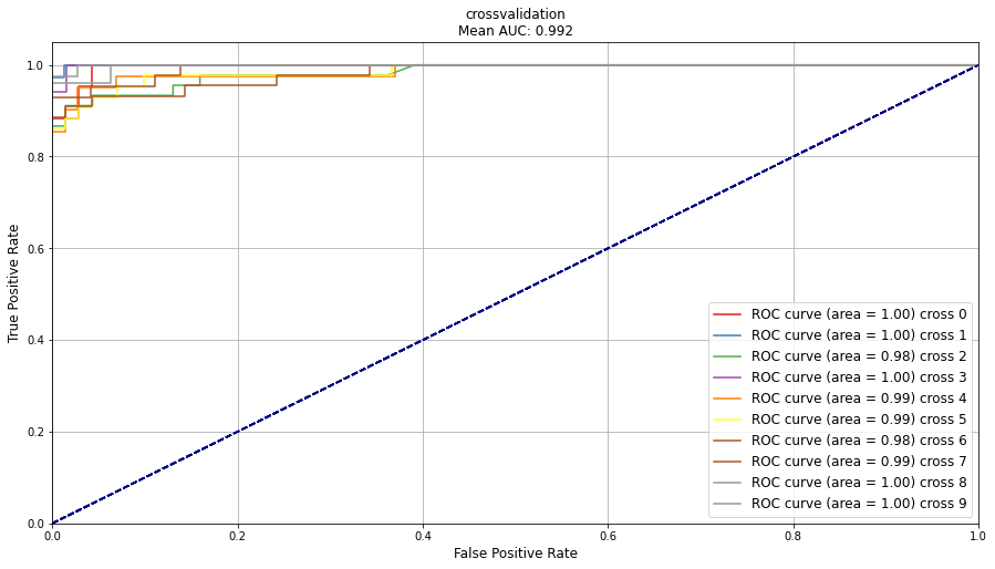
Cross validation
The classeval library provides an easy way of plotting multiple evaluations of crosses using the function classeval.classeval.plot_cross().
This function requires a dict that contains the evaluations from the two-class approach.
# Import library
import classeval as clf

# Load example dataset
X, y = clf.load_example('breast')
# Create empty dict to store the results
out = {}

# 10-fold crossvalidation
for i in range(0,10):
    # Random train/test split
    X_train, X_test, y_train, y_true = train_test_split(X, y, test_size=0.2)
    # Train model and make predictions on test set
    model = gb.fit(X_train, y_train)
    y_proba = model.predict_proba(X_test)[:,1]
    y_pred = model.predict(X_test)
    # Evaluate model and store in each evalution
    name = 'cross '+str(i)
    out[name] = clf.eval(y_true, y_proba, y_pred=y_pred, pos_label='malignant')

# After running the cross-validation, the ROC/AUC can be plotted as following:
clf.plot_cross(out, title='crossvalidation')
ROC/AUC 10-fold crossvalidation