Examples two-class model
In this example we are going to learn a model, and use the output y_true, y_proba and y_pred in classeval for the evaluation of the model.
# Import library
import classeval as clf

# Load example dataset
X, y = clf.load_example('breast')
X_train, X_test, y_train, y_true = train_test_split(X, y, test_size=0.2)

# Train model
model = gb.fit(X_train, y_train)
y_proba = model.predict_proba(X_test)[:,1]
y_pred = model.predict(X_test)
Now we can evaluate the model by:
# Evaluate
out = clf.eval(y_true, y_proba, pos_label='malignant')
Print some results to screen:
# Print AUC score
print(out['auc'])

# Print f1-score
print(out['f1'])

# Show some results
print(out['report'])
#
#                 precision    recall  f1-score   support
#
#          False       0.96      0.96      0.96        70
#           True       0.93      0.93      0.93        44
#
#       accuracy                           0.95       114
#      macro avg       0.94      0.94      0.94       114
#   weighted avg       0.95      0.95      0.95       114
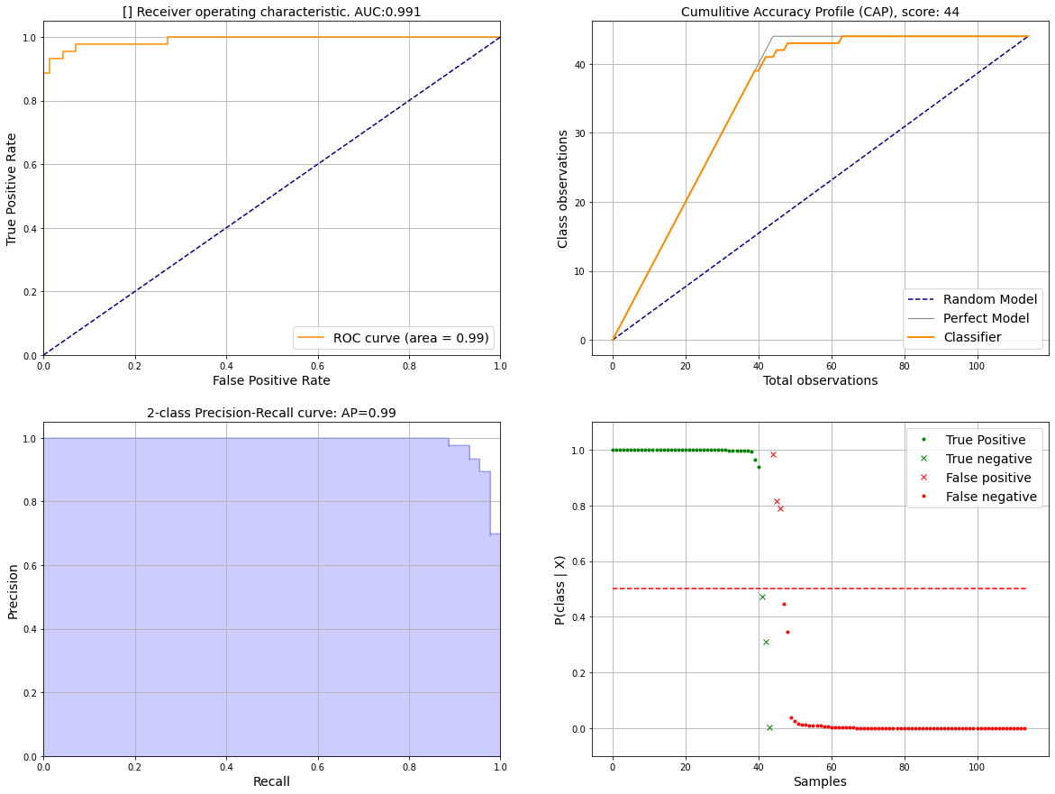
Plot by using classeval.classeval.plot():
- Four subplots are created:
top left: ROC curve
top right: CAP curve
bottom left: AP curve
bottom right: Probability curve
# Make plot
ax = clf.plot(out, figsize=(20,15), fontsize=14)
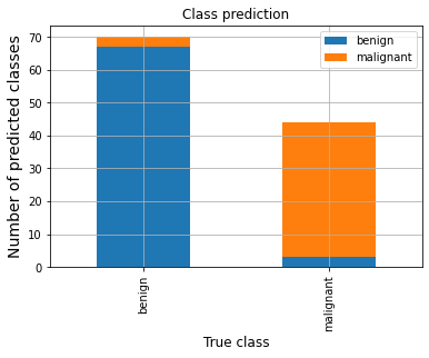
Class distribution in a bargraph
ROC in two-class
Plot ROC using:
# Compute ROC
out_ROC = clf.ROC.eval(y_true, y_proba, pos_label='malignant')

# Make plot
ax = clf.ROC.plot(out_ROC, title='Breast dataset')
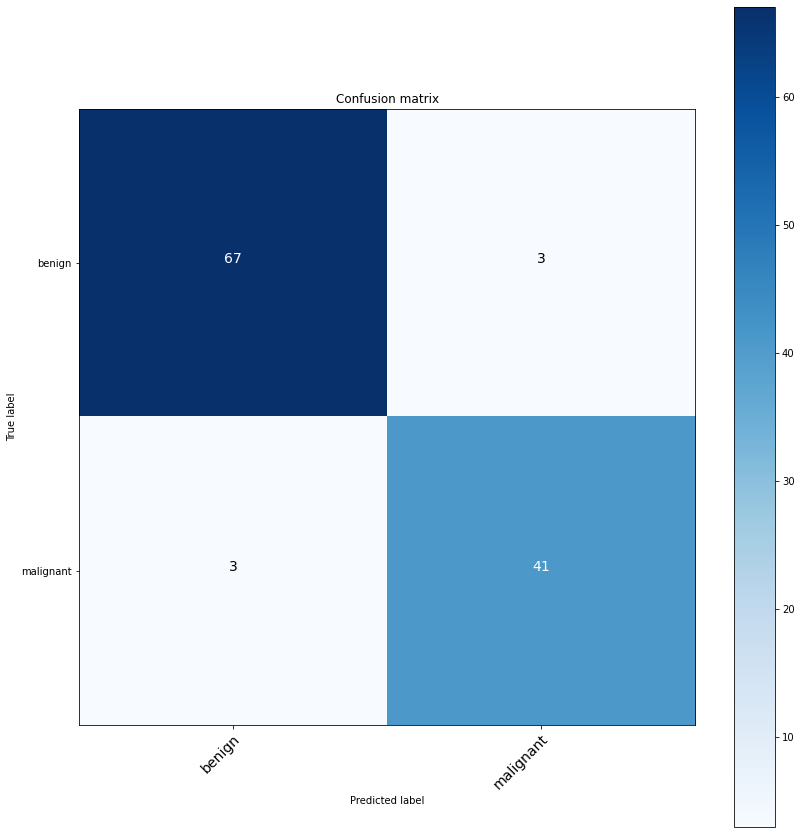
Confmatrix in two-class
It is also possible to plot only the confusion matrix:
# Compute confmatrix
out_CONFMAT = clf.confmatrix.eval(y_true, y_pred, normalize=True)

# Make plot
clf.confmatrix.plot(out_CONFMAT, fontsize=18)
Examples multi-class model
In this example we are going to learn a multi-class model, and use the output y_true, y_proba and y_pred in classeval for the evaluation of the model.
# Import library
import classeval as clf

# Load example dataset
X,y = clf.load_example('iris')
X_train, X_test, y_train, y_true = train_test_split(X, y, test_size=0.5)

# Train model
model = gb.fit(X_train, y_train)
y_pred = model.predict(X_test)
y_proba = model.predict_proba(X_test)
y_score = model.decision_function(X_test)
Lets evaluate the model results:
out = clf.eval(y_true, y_proba, y_score, y_pred)
Plot by using classeval.classeval.plot()
# Make plot
ax = clf.plot(out)
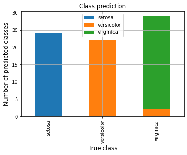
Class distribution in a bargraph
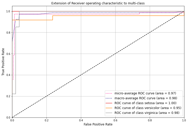
ROC in multi-class
ROC uses the same function as for two-class.
# ROC evaluation
out_ROC = clf.ROC.eval(y_true, y_proba, y_score)
ax = clf.ROC.plot(out_ROC, title='Iris dataset')
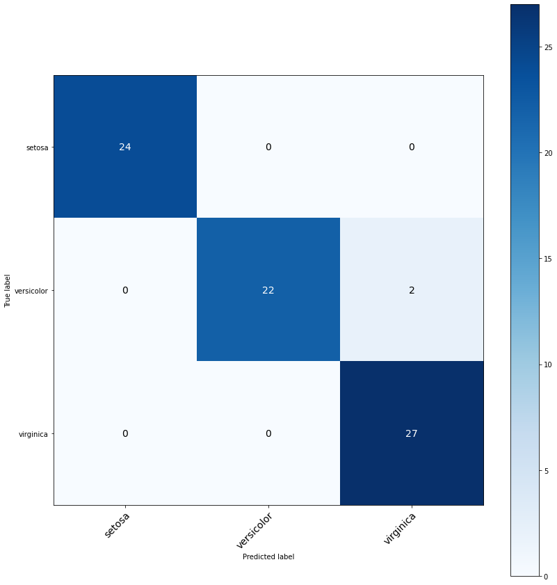
Confmatrix in multi-class
Confmatrix uses the same function as for two-class.
# Confmatrix evaluation
out_CONFMAT = clf.confmatrix.eval(y_true, y_pred, normalize=False)
ax = clf.confmatrix.plot(out_CONFMAT)
Confusion matrix
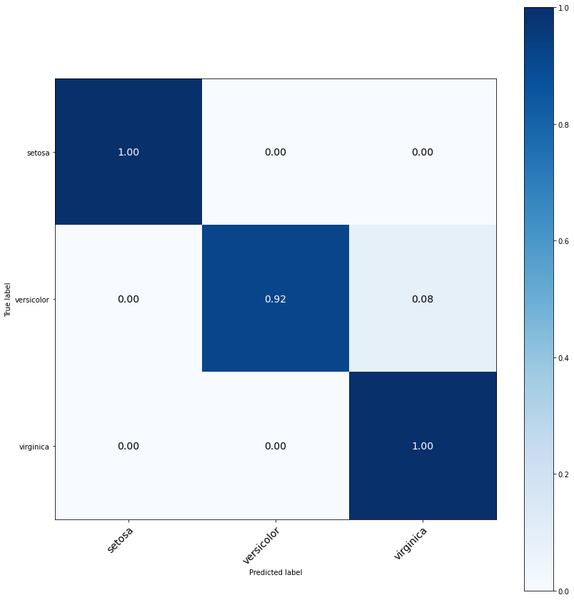
Normalized confusion matrix
# Confusion matrix
out_CONFMAT = clf.confmatrix.eval(y_true, y_pred, normalize=True)
# Plot
ax = clf.confmatrix.plot(out_CONFMAT)
Model Performance tweaking
It can be desired to tweak the performance of the model and thereby adjust, for example the number of False postives. With classeval it is easy to determine the most desired model.
Lets start with a simple model.
# Load example dataset
    X, y = clf.load_example('breast')
    X_train, X_test, y_train, y_true = train_test_split(X, y, test_size=0.2)

# Fit model
    model = gb.fit(X_train, y_train)
    y_proba = model.predict_proba(X_test)[:,1]
    y_pred = model.predict(X_test)
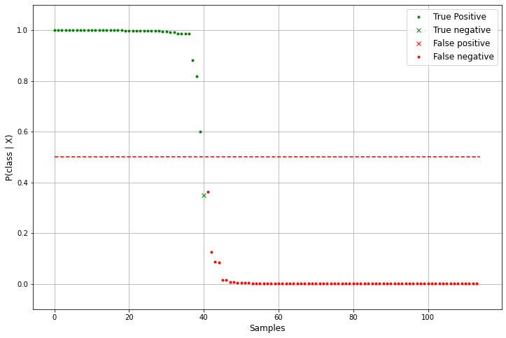
The default threshold value is 0.5 and gives these results:
# Set threshold at 0.5 (default)
out = clf.eval(y_true, y_proba, pos_label='malignant', threshold=0.5)

# [[73  0]
# [ 1 40]]

# Make plot
_ = clf.TPFP(out['y_true'], out['y_proba'], threshold=0.2, showfig=True, )
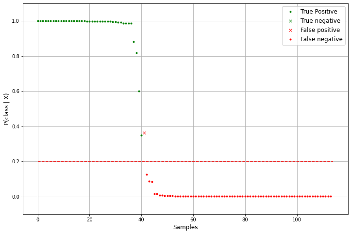
Lets adjust the model by setting the threshold differently:
# Set threshold at 0.2
out = clf.eval(y_true, y_proba, pos_label='malignant', threshold=0.2)

# [[72  1]
# [ 0 41]]

# Make plot
_ = clf.TPFP(out['y_true'], out['y_proba'], threshold=0.2, showfig=True, )
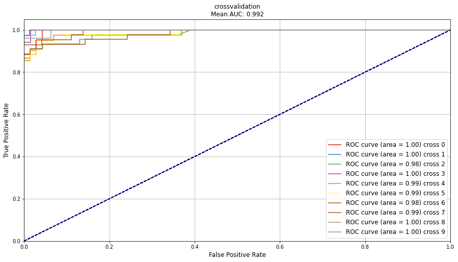
Cross-validation
Below is depicted an example of plotting cross-validation using classeval.
# Import library
import classeval as clf

# Load example dataset
X, y = clf.load_example('breast')
# Create empty dict to store the results
out = {}

# 10-fold crossvalidation
for i in range(0,10):
    # Random train/test split
    X_train, X_test, y_train, y_true = train_test_split(X, y, test_size=0.2)
    # Train model and make predictions on test set
    model = gb.fit(X_train, y_train)
    y_proba = model.predict_proba(X_test)[:,1]
    y_pred = model.predict(X_test)
    # Evaluate model and store in each evalution
    name = 'cross '+str(i)
    out[name] = clf.eval(y_true, y_proba, y_pred=y_pred, pos_label='malignant')

# After running the cross-validation, the ROC/AUC can be plotted as following:
clf.plot_cross(out, title='crossvalidation')