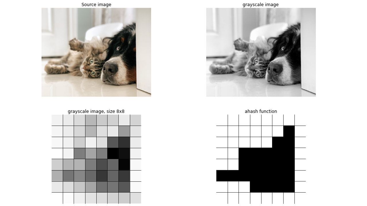
Average hash

After the decolorizing and scaling step, each pixel block is compared to the average (as the name suggests) of all pixel values of the image. In the example below, we will generate a 64-bit hash, which means that the image is scaled to 8×8 pixels. If the value in the pixel block is larger than the average, it gets value 1 (white) and otherwise a 0 (black). The final image hash is followed by flattening the array into a vector.

# Initialize with hash
model = Undouble(method='ahash')

# Import example
X = model.import_example(data='cat_and_dog')
imgs = model.import_data(X, return_results=True)

# Compute hash for a single image
hashs = model.compute_imghash(imgs['img'][0], to_array=False, hash_size=8)

# The hash is a binairy array or vector.
print(hashs)

# Plot the image using the undouble plot_hash functionality
model.results['img_hash_bin']
model.plot_hash(idx=0)

# Plot the image manually
fig, ax = plt.subplots(1, 2, figsize=(8,8))
ax[0].imshow(imgs['img'][0])
ax[1].imshow(hashs[0])

Average hash

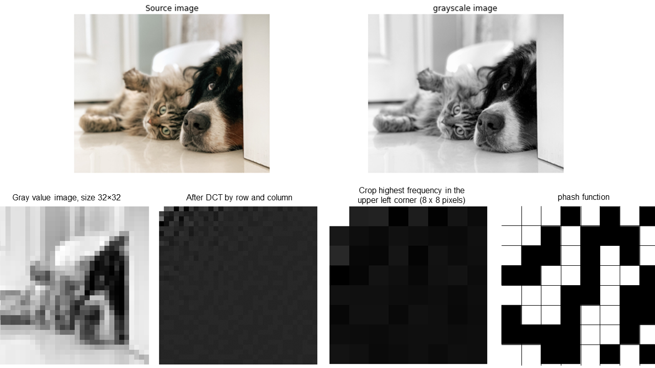
Perceptual hash

After the first step of decolorizing, a Discrete Cosine Transform (DCT) is applied; first per row and afterward per column. The pixels with high frequencies are cropped to 8 x 8 pixels. Each pixel block is then compared to the median of all gray values of the image. If the value in the pixel block is larger than the median, it gets value 1 and otherwise a 0. The final image hash is followed by flattening the array into a vector.

# Initialize with hash
model = Undouble(method='phash')

# Import example
X = model.import_example(data='cat_and_dog')
imgs = model.import_data(X, return_results=True)

# Compute hash for a single image
hashs = model.compute_imghash(imgs['img'][0], to_array=False, hash_size=8)

# The hash is a binairy array or vector.
print(hashs)

# Plot the image using the undouble plot_hash functionality
model.results['img_hash_bin']
model.plot_hash(idx=0)

# Plot the image manually
fig, ax = plt.subplots(1, 2, figsize=(8,8))
ax[0].imshow(imgs['img'][0])
ax[1].imshow(hashs[0])

Perceptual hash

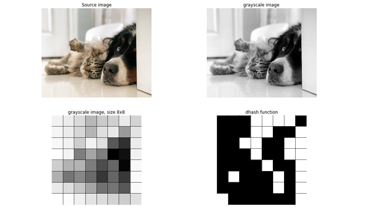
Differential hash

After the first step of decolorizing and scaling, the pixels are serially (from left to right per row) compared to their neighbor to the right. If the byte at position x is less than the byte at position (x+1), it gets value 1 and otherwise a 0. The final image hash is followed by flattening the array into a vector.

# Initialize with hash
model = Undouble(method='dhash')

# Import example
X = model.import_example(data='cat_and_dog')
imgs = model.import_data(X, return_results=True)

# Compute hash for a single image
hashs = model.compute_imghash(imgs['img'][0], to_array=False, hash_size=8)

# The hash is a binairy array or vector.
print(hashs)

# Plot the image using the undouble plot_hash functionality
model.results['img_hash_bin']
model.plot_hash(idx=0)

# Plot the image manually
fig, ax = plt.subplots(1, 2, figsize=(8,8))
ax[0].imshow(imgs['img'][0])
ax[1].imshow(hashs[0])

Differential hash

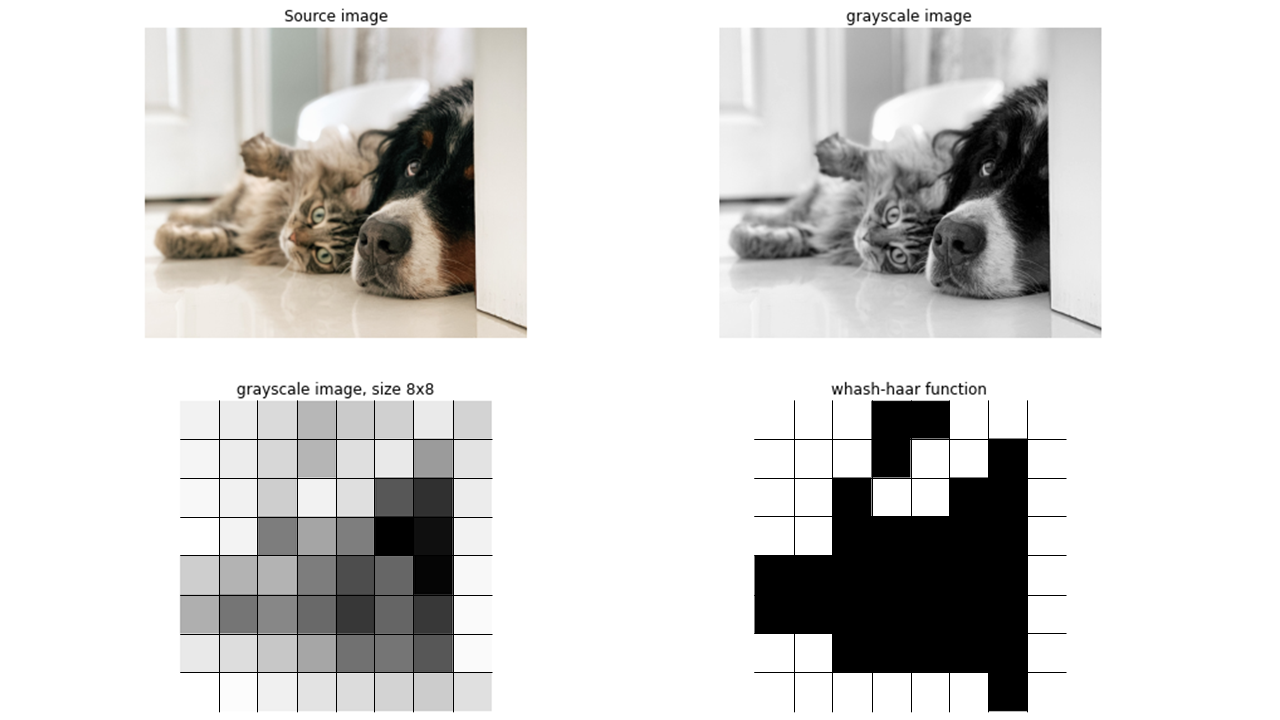
Haar wavelet hash

After the first step of decolorizing and scaling, a two-dimensional wavelet transform is applied to the image. Each pixel block is then compared to the median of all gray values of the image. If the value in the pixel block is larger than the median, it gets value 1 and otherwise a 0. The final image hash is followed by flattening the array into a vector.

# Initialize with hash
model = Undouble(method='whash-haar')

# Import example
X = model.import_example(data='cat_and_dog')
imgs = model.import_data(X, return_results=True)

# Compute hash for a single image
hashs = model.compute_imghash(imgs['img'][0], to_array=False, hash_size=8)

# The hash is a binairy array or vector.
print(hashs)

# Plot the image using the undouble plot_hash functionality
model.results['img_hash_bin']
model.plot_hash(idx=0)

# Plot the image manually
fig, ax = plt.subplots(1, 2, figsize=(8,8))
ax[0].imshow(imgs['img'][0])
ax[1].imshow(hashs[0])

Haar wavelet hash

Crop-resistant hash

The Crop resistant hash is implemented as described in the paper “Efficient Cropping-Resistant Robust Image Hashing”. DOI 10.1109/ARES.2014.85. This algorithm partitions the image into bright and dark segments, using a watershed-like algorithm, and then does an image hash on each segment. This makes the image much more resistant to cropping than other algorithms, with the paper claiming resistance to up to 50% cropping, while most other algorithms stop at about 5% cropping.

# Import library
from undouble import Undouble

# Init with default settings
model = Undouble()

# Import example data
targetdir = model.import_example(data='flowers')

# Importing the files files from disk, cleaning and pre-processing
model.import_data(targetdir)

# Compute image-hash
model.compute_hash(method='crop-resistant-hash')

# Find images with image-hash <= threshold
results = model.group(threshold=5)

# Plot the images
model.plot()

# Print the output for demonstration
print(model.results.keys())

# The detected groups
model.results['select_pathnames']
model.results['select_scores']
model.results['select_idx']

# Plot the hash for the first group
model.plot_hash(filenames=model.results['filenames'][model.results['select_idx'][0]])

Plot image hash

All examples are created using the underneath code:

# pip install imagesc

import cv2
from scipy.spatial import distance
import numpy as np
import matplotlib.pyplot as plt
from imagesc import imagesc
from undouble import Undouble

methods = ['ahash', 'dhash', 'whash-haar']

for method in methods:
    # Average Hash
    model = Undouble(method=method, hash_size=8)
    # Import example data
    targetdir = model.import_example(data='cat_and_dog')
    # Grayscaling and scaling
    model.import_data(targetdir)
    # Compute image for only the first image.
    hashs = model.compute_imghash(model.results['img'][0], to_array=True)
    # Compute the image-hash
    print(method + ' Hash:')
    image_hash = ''.join(hashs[0].astype(int).astype(str).ravel())
    print(image_hash)

    # Import image for plotting purposes
    img_g = cv2.imread(model.results['pathnames'][0], cv2.IMREAD_GRAYSCALE)
    img_r = cv2.resize(img_g, (8, 8), interpolation=cv2.INTER_AREA)

    # Make the figure
    fig, ax = plt.subplots(2, 2, figsize=(15, 10))
    ax[0][0].imshow(model.results['img'][0][..., ::-1])
    ax[0][0].axis('off')
    ax[0][0].set_title('Source image')
    ax[0][1].imshow(img_g, cmap='gray')
    ax[0][1].axis('off')
    ax[0][1].set_title('grayscale image')
    ax[1][0].imshow(img_r, cmap='gray')
    ax[1][0].axis('off')
    ax[1][0].set_title('grayscale image, size %.0dx%.0d' %(8, 8))
    ax[1][1].imshow(hashs[0], cmap='gray')
    ax[1][1].axis('off')
    ax[1][1].set_title(method + ' function')

    # Compute image hash for the 10 images.
    hashs = model.compute_imghash(model, to_array=False)

    # Compute number of differences across all images.
    adjmat = np.zeros((hashs.shape[0], hashs.shape[0]))
    for i, h1 in enumerate(hashs):
        for j, h2 in enumerate(hashs):
            adjmat[i, j] = np.sum(h1!=h2)

    # Compute the average image-hash difference.
    diff = np.mean(adjmat[np.triu_indices(adjmat.shape[0], k=1)])
    print('[%s] Average difference: %.2f' %(method, diff))

    # Make a heatmap to demonstrate the differences between the image-hashes
    imagesc.plot(hashs, cmap='gray', col_labels='', row_labels=model.results['filenames'], cbar=False, title=method + '\nAverage difference: %.3f' %(diff), annot=True)

---

---