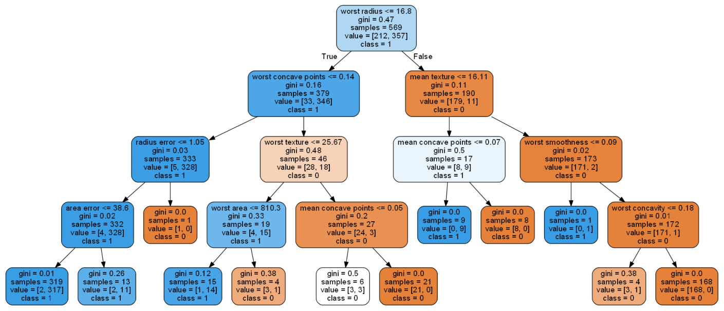
RandomForest
In the following example we learn a simple RandomForest model and plot the tree.
# Library to for model
from sklearn.tree import DecisionTreeClassifier
from sklearn import datasets

# Load example data
data = datasets.load_breast_cancer()

# Learn model
model = DecisionTreeClassifier(max_depth=4, random_state=0).fit(data.data, data.target)

# Import treeplot library
import treeplot as tree

# Plot the tree
ax = tree.plot(model, featnames=data.feature_names)
|
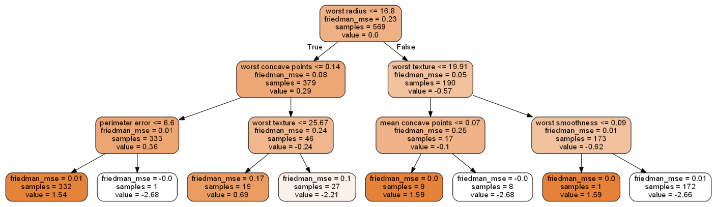
GradientBoostingClassifier
In the following example we learn a simple GradientBoostingClassifier model and plot the tree.
# Library to for model
from sklearn.ensemble import GradientBoostingClassifier
from sklearn import datasets

# Load example data
data = datasets.load_breast_cancer()

# Learn model
model = GradientBoostingClassifier().fit(data.data, data.target)

# Import treeplot library
import treeplot as tree

# Plot the tree
ax = tree.plot(model, featnames=data.feature_names)
|
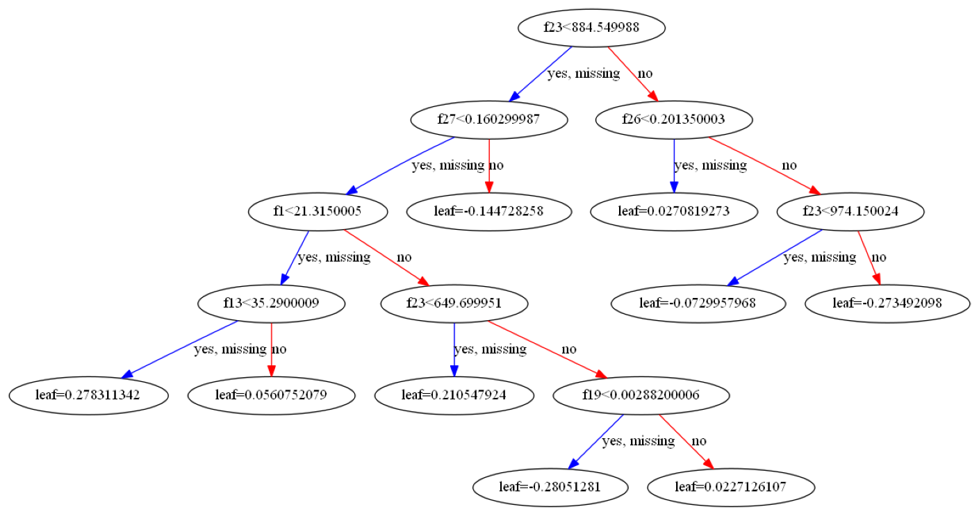
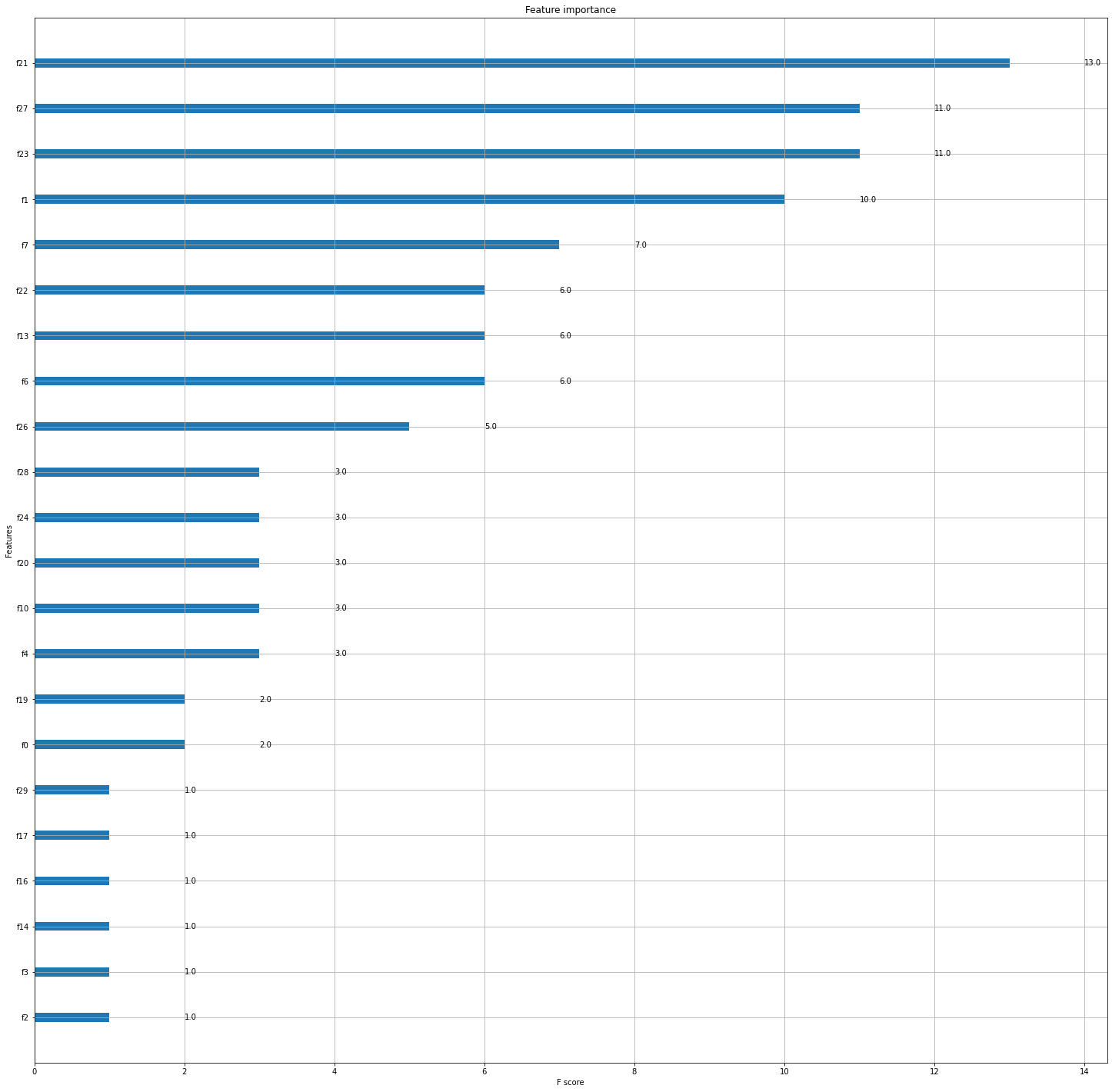
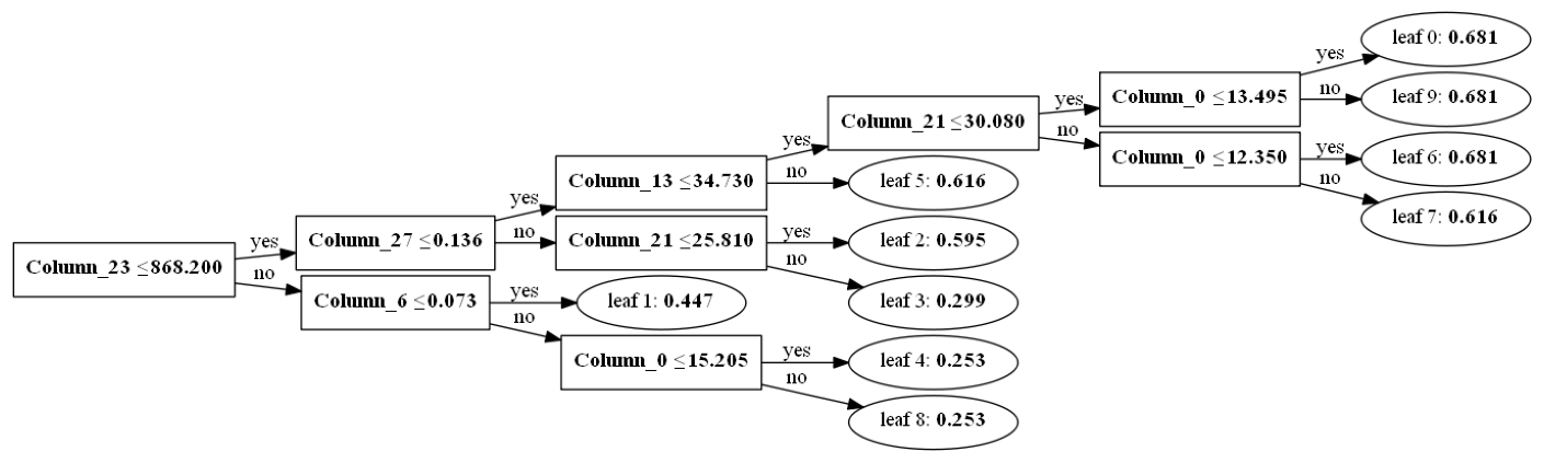
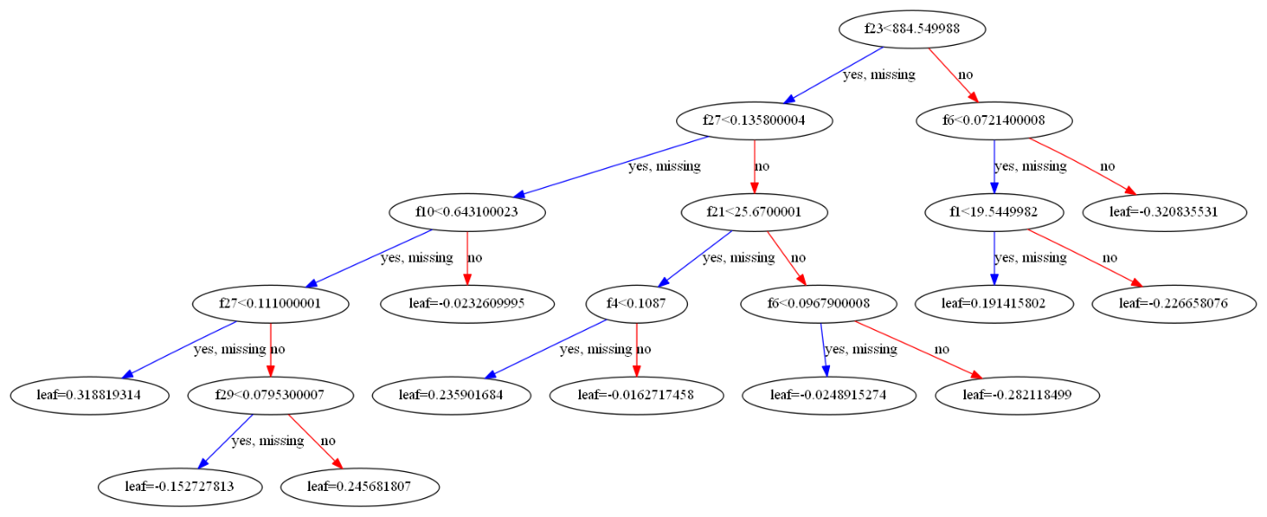
XGboost
In the following example we learn a simple XGboost model and plot the tree.
# Library to for model
import xgboost as xgb
from sklearn import datasets

# Load example data
data = datasets.load_breast_cancer()

# Learn model
model = xgb.XGBClassifier(use_label_encoder=False, n_estimators=10, max_depth=5, random_state=0, eval_metric='logloss').fit(data.data, data.target)

# Import treeplot library
import treeplot as tree

# Plot the tree
ax = tree.plot(model, featnames=data.feature_names)
|
|

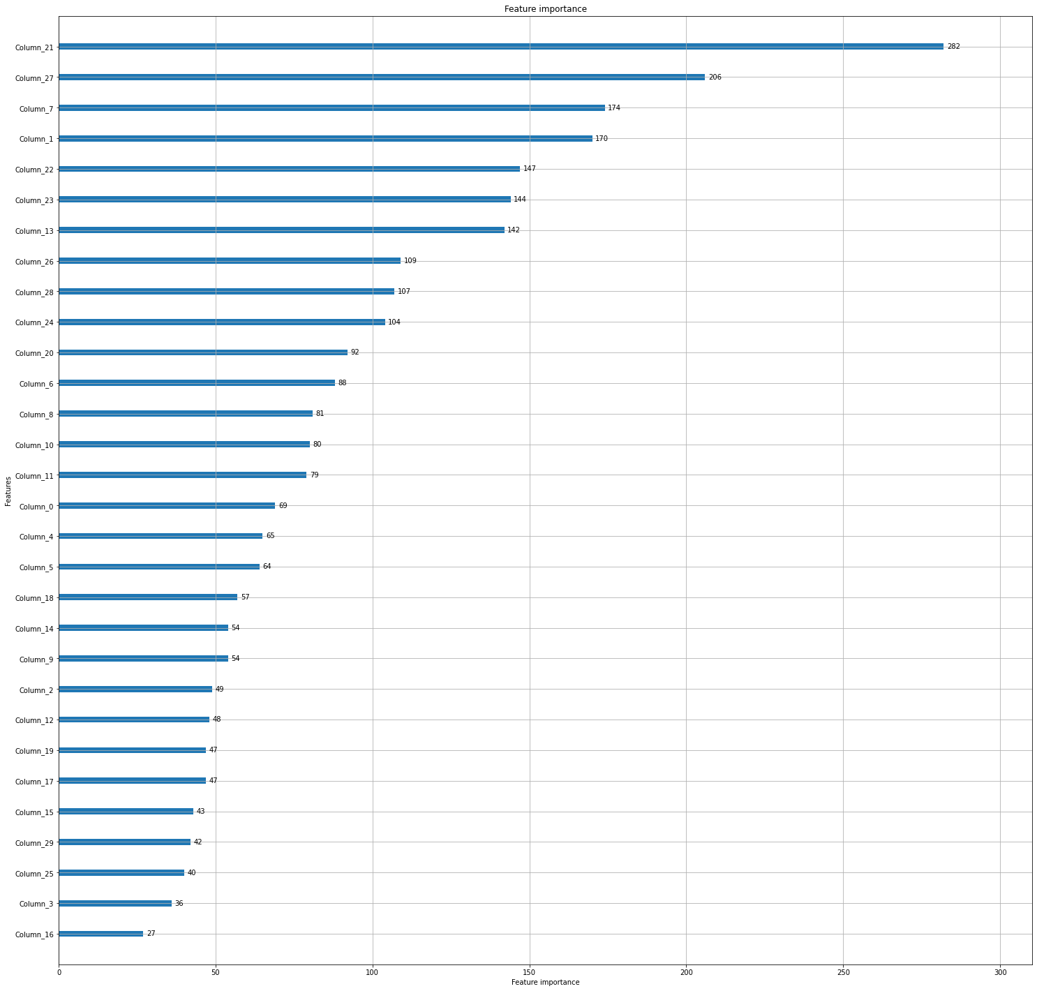
LightBM
In the following example we learn a simple LightBM model and plot the tree.
# Library to for model
from lightgbm import LGBMClassifier
from sklearn import datasets

# Load example data
data = datasets.load_breast_cancer()

# Learn model
model = LGBMClassifier().fit(data.data, data.target)

# Import treeplot library
import treeplot as tree

# Plot the tree
ax = tree.plot(model, featnames=data.feature_names)
|
|
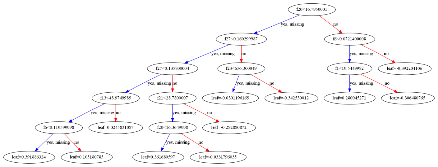
Plot second best Tree and other Trees
The opimization proces in the tee models will return the best performing models. However, other learned trees are also available and can be easily plotted. Let’s vizualize the second and third best tree.
# Library to for model
import xgboost as xgb
from sklearn import datasets

# Load example data
data = datasets.load_breast_cancer()

# Learn model
model = xgb.XGBClassifier(use_label_encoder=False, n_estimators=10, max_depth=5, random_state=0, eval_metric='logloss').fit(data.data, data.target)

# Import treeplot library
import treeplot as tree

# Plot the tree
ax = tree.plot(model, featnames=data.feature_names, num_trees=2)
ax = tree.plot(model, featnames=data.feature_names, num_trees=5)
|
|
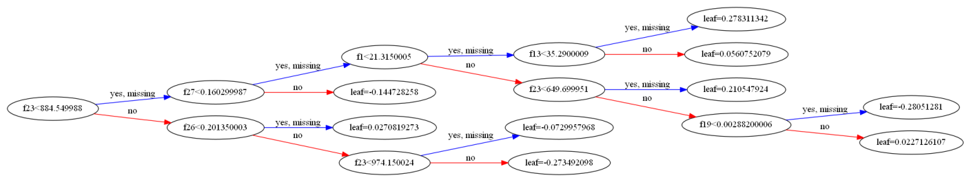
XGBoost Horizontal vs. Vertical
Changing the horizontal or vertical plotting can only be for XGboost.
# Library to for model
import xgboost as xgb
from sklearn import datasets

# Load example data
data = datasets.load_breast_cancer()

# Learn model
model = xgb.XGBClassifier(use_label_encoder=False, n_estimators=10, max_depth=5, random_state=0, eval_metric='logloss').fit(data.data, data.target)

# Import treeplot library
import treeplot as tree

# Plot the tree
ax = tree.plot(model, featnames=data.feature_names, plottype='vertical')
ax = tree.plot(model, featnames=data.feature_names, plottype='horizontal')
|
|